Discriminative Predictive Coding (Whittington & Bogacz; 2017)

In this exhibit, we will see how a classifier can be created based on predictive coding. This exhibit model effectively reproduces some of the results reported (Whittington & Bogacz, 2017) [1]. The model code for this exhibit can be found here.

Note: You will need to unzip the MNIST arrays in data/mnist.zip to the folder data/ to work through this exhibit/walkthrough.

The Predictive Coding Network (PCN)

The discriminative predictive coding network (PCN) is a hierarchical neuronal model that seeks to predict the label y ($\mathbf{y}$; typically a one-hot encoded label) of a given sensory input data point x ($\mathbf{x}$). The PCN model of [1] showed that constructing a multi-layer system composed of layers of stateful neural processing units, where one layer of neurons would locally predict the activities of the ones (situated) above them, resulted in an effective yet more biologically-plausible classifier, as compared to deep neural networks trained with backpropagation of errors (or backprop). Furthermore, [1] showed that the underlying dynamics of the PCN could be shown to recover the updates to synaptic weights produced by backprop under certain assumptions/conditions.

In ngc-learn, building the PCN requires working with the library’s graded neurons, i.e., those that follow dynamics without spikes/discrete action potentials, specifically the RateCell and the GaussianErrorCell components. In effect, to construct a two hidden layer model of the form of [1], one will wire together four layers of RateCell’s, i.e., z0 ($\mathbf{z}^0$), z1 ($\mathbf{z}^1$), z2 ($\mathbf{z}^2$), z3 ($\mathbf{z}^3$), with three hebbian synapses, i.e., W1 ($\mathbf{W}^1$), W2 ($\mathbf{W}^1$), W3 ($\mathbf{W}^1$). Inference conducted in accordance with predictive coding mechanics generally follows a message-passing scheme where local prediction errors – the error/mismatch activities associated with each layer’s guess of the activities of the one above it – are passed up and down via local feedback synaptic connections in order to produce updates to the neuronal activities themselves. Notice that this is much akin to the E-step of expectation-maximization (E-M) [2]. This message-passing is done typically for several steps in time and, after these dynamics are iteratively run several times, the synaptic weight updates are computed for each layer’s associated predictive synapses (W1, W2, and W3) using two-factor Hebbian rules.

Formally, the above means, in ngc-learn, that each layer of neuronal dynamics can be characterized by the following single ordinary differential equation (ODE):

\[ \tau_m \frac{\partial \mathbf{z}^\ell_t}{\partial t} = (-\gamma \mathbf{z}^\ell_t + \mathbf{h}^\ell_t), \; \text{where} \; \mathbf{h}^\ell_t = -\mathbf{e}^\ell_t + (\mathbf{W}^{\ell+1})^T \cdot \mathbf{e}^{\ell+1}_t \]

where $()^T$ denotes the matrix transpose and $\cdot$ denotes matrix/vector multiplication. Since there is no layer above it and it will only ever be clamped to the label $\mathbf{y}$ (during training), $\mathbf{z}^\ell_t=3$’s dynamics ultimately reduce to $\mathbf{z}^3_t = \mathbf{y}$, i.e., this means we set the target output activity to be equal to the label. Furthermore, the bottom layer $\mathbf{z}^0_t$ will always be clamped to the sensory input, e.g., a pixel image, so it also reduces to $\mathbf{z}^0 = \mathbf{x}$ (this means that we set the input layer to be equal to the data).[1] These two simplifications means we only need to run the dynamics for neuronal layers $\mathbf{z}^1$ and $\mathbf{z}^2$ via Euler integration (which is what the RateCell does by default).

The only other key aspect to define in the above ODE is what $\mathbf{e}^\ell_t$ means. This is known in ngc-learn as an “error cell”, which is another type of graded neuron component and is, for the purposes of constructing the model of [1], defined as:

\[ \mathbf{e}^\ell_t = (\mathbf{z}^\ell_t - \mu^\ell_t), \; \text{where} \; \mu^\ell_t = \mathbf{W}^\ell \cdot \phi^{\ell-1}(\mathbf{z}^{\ell-1}) \]

given that it is the first derivative (with respect to the prediction mean $\mu^\ell_t$) of a Gaussian log likelihood functional $\mathcal{F}^\ell$, with fixed unit variance, applied locally to measure the discrepancy between the actual neural activity at layer $\ell$ – $\mathbf{z}^\ell_t$ – and the predicted neural activity $\mu^\ell_t$. You will notice that the equation $\mu^\ell_t = \mathbf{W}^\ell \cdot \phi^{\ell-1}(\mathbf{z}^{\ell-1})$ depicts how a local prediction is made from layer $\ell-1$ about the activity values in layer $\ell$, where $\phi^{\ell-1}$ is an elementwise activation function applied to the neuronal activity values (note that the PCN model in ngc-learn sets these to sigmoid).[2]

The next important part in characterizing a PCN is its synaptic dynamics, which, after running the above equations for several steps in time, amounts to a single application of the following ODE (for each weight matrix W1, W2, and W3):

\[ \tau_w \frac{\partial \mathbf{W}^\ell_{t_j}}{\partial {t_j}} = -\lambda \mathbf{W}^\ell_{t_j} + \mathbf{e}^\ell \cdot (\phi^{\ell-1}(\mathbf{z}^{\ell-1}))^T \]

where we use $t_j$ to indicate that the time-scale of the updates for any synaptic weight matrix $\mathbf{W}^\ell$ is slower than those of the neuronal activities described earlier.

The last part for constructing an effective PCN for classification is simply determining how the initial conditions are set for the neurons in layers $\ell = 1$ and $\ell = 2$. Much as in [1], this is done by clamping the input layer to sensory data, i.e., $\mathbf{z}^0 = \mathbf{x}$, clamping the output layer to label data $\mathbf{z}^3 = \mathbf{y}$, and initializing $\mathbf{z}^1$ and $\mathbf{z}^2$ to values that are produced via feedforward pass/sweep (or “ancestral projection pass”) from the input layer to output layer via:

\[\begin{split} \mu^1_t &= \mathbf{W}^1 \cdot \mathbf{z}^0, \; \mathbf{z}^1 = \phi^1(\mu^1_t) \\ \mu^2_t &= \mathbf{W}^2 \cdot \mathbf{z}^1, \; \mathbf{z}^2 = \phi^2(\mu^2_t) \\ \mu^3_t &= \mathbf{W}^3 \cdot \mathbf{z}^2 \end{split}\]

which also gets us our initial local predictions for free (same goes for the error values, which are, at initialization, $\mathbf{e}^1 = 0$, $\mathbf{e}^2 = 0$, and $\mathbf{e}^3 = \mathbf{z}^3_t - \mu^3_t$). (Note: the above equations are simply run for test-time when a label is not present to obtain a fast prediction of input samples in the test-set and to measure model generalization ability.)

In the figure below, we graphically depict what the simulated PCN and its corresponding conditional generative model (ancestral projection graph) look like (the blue dashed arrow just points outs that the layer mu1 of the feedforward sweep step is used to initialize the neuronal activities of z1 in the PCN model’s dynamics). Note that mu1 is $\mu^1_t$, mu2 is $\mu^2_t$, and mu3 is $\mu^3_t$ while z^1_t is $\mathbf{z}^1_t$, z^2_t is $\mathbf{z}^2_t$, and z^2_t is $\mathbf{z}^3_t$ (z^0_t is the input layer $\mathbf{z}^0$).

Constructing the above model dynamics and initial conditions, as well as simulating these over multiple passes through the MNIST database, is what is done in the model exhibit code for the PCN. Effectively, most of the central configuration/hyper-parameters values can be done through the model exhibit’s constructor (relevant snippet from train_pcn.py shown below):

model = PCN(subkeys[1], x_dim, y_dim, hid1_dim=512, hid2_dim=512, T=20,
            dt=1., tau_m=20., act_fx="sigmoid", eta=0.001, exp_dir="exp",
            model_name="pcn")

where the integration time constant for the Euler integration of the neuronal dynamics is set to 1 millisecond (ms) which are run for T = 20 (E-)steps before synaptic weights are updated with the Hebbian ODE shown above. Also, much as in [1], the Adam adaptive learning rate (with global learning rate eta = 0.001) is used to apply the Hebbian adjustments to the synaptic weight values.

Note that the PCN exhibit model constructor provides, among several model and task-specific functions and convenience routines, a key function called process, which takes in sensory input and labels and runs the full E-M dynamics described earlier. In this function, there is an argument called adapt_synapses which, if set to True, will run the model’s settling dynamics and perform the synaptic update steps after T E-steps have been simulated; however, if it is set to False, the learning dynamics are turned off and only the output prediction $\mu^3_t$ (mu3) is read out (the label is not used).

Running the PCN Model

To train the PCN classifier described above, go to the exhibits/pc_discrim sub-folder (this step assumes that you have git cloned the model museum repo code), and execute the PCN’s training script from the command line as follows:

$ ./sim.sh ## default verbosity level set to 0

which will execute a training process using an experimental configuration very similar to (Whittington & Bogacz, 2017). After your model finishes training you should see a validation score and output similar[4] to the one below:

------------------------------------
 Trial.sim_time = 0.07287026127179463 h  (262.3329405784607 sec)  Best Acc = 0.9821000695228577

You will also notice that in the experimental output folder created for you by the script – /exp/ – which contains several saved arrays as well as your learned ngc-learn model, saved to disk for you as follows:

/exp/nll.npy (the model’s predictive output negative log likelihood measurements),
/exp/efe.npy (the PCN’s free energy measurements),
/exp/acc.npy (the model’s development accuracy measurements), and,
/exp/trAcc.npy (the model’s training accuracy measurements)).

To use your saved model and examine its performance on the MNIST test-set, you can execute the evaluation script like so:

$ python analyze_pcn.py  --dataX="../data/mnist/testX.npy" \
                         --dataY="../data/mnist/testY.npy"

which should result in an output similar what is shown below:

------------------------------------
=> NLL = 0.07531584054231644  Acc = 0.9803001284599304

Desirably, our out-of-sample results on both the validation and test-set corroborate the measurements reported in (Whittington & Bogacz, 2017) [1], i.e., less than 2% validation error was reported and our simulation yields a validation accuracy of 0.9821 * 100 = 98.21% (or 1.79% error) and a test accuracy of 0.9803 * 100 = 98.03% (or about 1.97% error), even though our predictive processing classifier differs in a minor ways.[3]

Furthermore, running the analyze_pcn.py script as above also produces, locally in your experimental directory exp/, a t-SNE visualization of your PCN’s penultimate layer of neuronal activities (its “latent codes” in the layer below the predictive output layer). You should see a t-SNE plot (named exp/pcn_latents.jpg) similar to the one below:

As can be seen in the plot above, the PCN’s latents look like they have roughly clustered themselves based on digit category (i.e., where something is zero versus whether it is a two, etc.), which is what we would expect given that the PCN directly uses the labels to drive the error cells at the very top layer (at $\mathbf{e}^3) during training.

Finally, since the model exhibit training code collects your model’s training and validation likelihood measurements at the end of each pass through the data (i.e., “epoch”), you can write some Python code to plot the model’s learning curves like so:

import matplotlib
import matplotlib.pyplot as plt
import matplotlib.patches as mpatches
import numpy as np

colors = ["red", "blue"]
# post-process learning curve data
y = (1.0 - np.load("exp/trAcc.npy")) * 100. ## training measurements
vy = (1.0 - np.load("exp/acc.npy")) * 100. ## dev measurements
x_iter = np.asarray(list(range(0, y.shape[0])))
## make the plots with matplotlib
fontSize = 20
plt.plot(x_iter, y, '-', color=colors[0])
plt.plot(x_iter, vy, '-', color=colors[1])
plt.xlabel("Epoch", fontsize=fontSize)
plt.ylabel("Classification Error", fontsize=fontSize)
plt.grid()
## construct the legend/key
loss = mpatches.Patch(color=colors[0], label='Train Acc')
vloss = mpatches.Patch(color=colors[1], label='Dev Acc')
plt.legend(handles=[loss, vloss], fontsize=13, ncol=2,borderaxespad=0, frameon=False,
           loc='upper center', bbox_to_anchor=(0.5, -0.175))
plt.tight_layout()
plt.savefig("exp/pcn_mnist_curves.jpg") ## save plot to disk
plt.clf()

which should produce a set of learning curves as below:

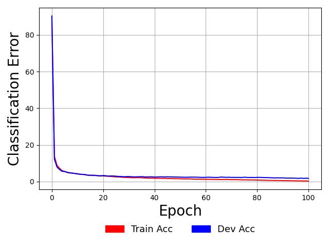
As observed in the plot above, this PCN classifier begins to overfit the training sample nearly perfectly, as indicated by the fact that the blue validation Dev Acc curve is a bit higher than the red Acc learning curve. Note that these reported accuracy measurements come from using the ancestral projection graph (the initialization step of the settling process) that we used to start the E-M process of the discriminative PCN system, meaning that we could deploy the projection graph itself as a probabilistic neuronal model of p(y|x).

Aside: Inspecting the PCN’s Free Energy

You will notice that, among your simulation code’s outputs in the /exp/ folder, is an array called efe.npy. This contains the PCN’s measured (expected) free energy, tracked cumulatively across the entire training dataset, at the end of each epoch. Plotting this array (with code similar to what was shown above for the learning curves) gives:

This plot simply shows that the entire PCN system can be shown to optimizing a global objective function, i.e., the full free energy $\mathcal{F} = \mathcal{F}^1 + \mathcal{F}^2 + \mathcal{F}^3$ (more generally, this $\mathcal{F} = \sum^L_{\ell=1} \mathcal{F}^\ell$, where we saw earlier that the first derivative of $\mathcal{F}^\ell$ was what gave us our error cell equation for layer $\ell$). Indeed, since we see that our free energy curve approaches zero (coming from very low negative values) in the above plot, our PCN is optimizing the full free energy $\mathcal{F}$. Note that, while it would not be easy to tell by visual inspection of the above plot, the final free energy reached is -1.9853954 (nats).

Computing Hardware Note:

This tutorial was tested and run on an Ubuntu 22.04.2 LTS operating system using an NVIDIA GeForce RTX 2070 GPU with CUDA Version: 12.1 (Driver Version: 530.41.03). Note that the times reported in any tutorial screenshot/console snippets were produced on this system.

References

[1] Whittington, James CR, and Rafal Bogacz. “An approximation of the error backpropagation algorithm in a predictive coding network with local hebbian synaptic plasticity.” Neural computation 29.5 (2017): 1229-1262.
[2] Dempster, Arthur P., Nan M. Laird, and Donald B. Rubin. “Maximum likelihood from incomplete data via the EM algorithm.” Journal of the royal statistical society: series B (methodological) 39.1 (1977): 1-22.