Reinforcement Learning through a Spiking Controller (Chevtchenko et al.; 2020)
In this exhibit, we will see how to construct a simple biophysical model for reinforcement learning with a spiking neural network and modulated spike-timing-dependent plasticity. This model incorporates a mechanisms from several different models, including the constrained RL-centric SNN of [1] as well as some simplifications of the structures used within the SNN of [2]. The model code for this exhibit can be found here.
Modeling Operant Conditioning through Modulation
Operant conditioning refers to the idea that there are environmental stimuli that can either increase or decrease the occurrence of (voluntary) behaviors; in other words, positive stimuli can lead to future repeats of a certain behavior whereas negative stimuli can lead to (i.e., punish) a decrease in future occurrences. Ultimately, operant conditioning, through consequences, shapes voluntary behavior where actions followed by rewards are repeated and actions followed by punished/negative outcomes diminish.
In this lesson, we will model very simple case of operant conditioning for a neuronal motor circuit used to engage in the navigation of a simple maze. The maze’s design will be the rat T-maze and the “rat” will be allowed to move, at a particular point in the maze, in one of four directions (up/North, down/South, left/West, and right/East). A positive reward will be supplied to our rat neuronal circuit if it makes progress towards the direction of food (placed in the upper right corner of the T-maze) and a negative reward will be provided if fails to make progress/gets stuck, i.e., a dense reward functional will be employed. For the exhibit code that goes with this lesson, an implementation of this T-maze environment is provided, modeled in the same style/with the same agent API as the OpenAI gymnasium.
Reward-Modulated Spike-Timing-Dependent Plasticity (R-STDP)
Although spike-timing-dependent plasticity (STDP) and reward-modulated STDP (MSTDP) are covered and analyzed in detail in the ngc-learn set of tutorials, we will briefly review the evolution of synaptic strengths as prescribed by modulated STDP with eligibiility traces here. In effect, STDP prescribes changes in synaptic strength according to the idea that neurons that fire together, wire together, except that timing matters (a temporal interpretation of basic Hebbian learning). This means that, assuming we are able to record the times of pre-synaptic and post-synaptic neurons (that a synaptic cable connects), we can, at any time-step \(t\), produce an adjustment \(\Delta W_{ij}(t)\) to a synapse via the following pair of correlational rules:
where \(s_j\) is the spike recorded at time \(t\) of the post-synaptic neuron \(j\) (and \(x_j\) is an exponentially-decaying trace that tracks its spiking history) and \(s_i\) is the spike recorded at time \(t\) of the pre-synaptic neuron \(i\) (and \(x_i\) is an exponentially-decaying trace that tracks its pulse history). STDP, as shown in a very simple format above, effectively can be described as balancing two types of alterations to a synaptic efficacy – long-term potentiation (the first term, which increases synaptic strength) and long-term depression (the second term, which decreases synaptic strength).
Modulated STDP is a three-factor variant of STDP that multiplies the final synaptic update by a third signal, e.g., the modulatory signal is often a reward (dopamine) intensity value (resulting in reward-modulated STDP). However, given that reward signals might be delayed or not arrive/be available at every single time-step, it is common practice to extend a synapse to maintain a second value called an “eligibility trace”, which is effectively another exponentially-decaying trace/filter (instantiated as an ODE that can be integrated via the Euler method or related tools) that is constructed to track a sequence of STDP updates applied across a window of time. Once a reward/modulator signal becomes available, the current trace is multiplied by the modulator to produce a change in synaptic efficacy. In essence, this update becomes:
where \(r(t)\) is the dopamine supplied at some time \(t\) and \(\nu\) is some non-negative global learning rate. Note that MSTDP with eligibility traces (MSTDP-ET) is agnostic to the choice of local STDP/Hebbian update used to produce \(\Delta W_{ij}(t)\) (for example, one could replace the trace-based STDP rule we presented above with BCM or a variant of weight-dependent STDP).
The Spiking Neural Circuit Model
In this exhibit, we build one of the simplest possible spiking neural networks (SNNs) one could design to tackle a simple maze navigation problem such as the rat T-maze; specifically, a three-layer SNN where the first layer is a Poisson encoder and the second and third layers contain sets of recurrent leaky integrate-and-fire (LIF) neurons. The recurrence in our model is to be non-plastic and constructed such that a form of lateral competition is induced among the LIF units, i.e., LIF neurons will be driven by a scaled Hollow-matrix initialized recurrent weight matrix (which will multiply spikes encountered at time \(t - \Delta t\) by negative values), which will (quickly yet roughly) approximate the effect of inhibitory neurons. For the synapses that transmit pulses from the sensory/input layer to the second layer, we will opt for a non-plastic sparse mixture of excitatory and inhibitory strength values (much as in the model of [1]) to produce a reasonable encoding of the input Poisson spike trains. For the synapses that transmit pulses from the second layer to the third (control/action) layer, we will employ MSTDP-ET (as shown in the previous section) to adjust the non-negative efficacies in order to learn a basic reactive policy. We will call this very simple neuronal model the “reinforcement learning SNN” (RL-SNN).
The SNN circuit will be provided raw pixels of the T-maze environment (however, this view is a global view of the entire maze, as opposed to something more realistic such as an egocentric view of the sensory space), where a cross “+” marks its current location and an “X” marks the location of the food substance/goal state. Shown below is an image to the left depicting a real-world rat T-maze whereas to the right is our implementation/simulation of the T-maze problem (and what our SNN circuit sees at the very start of an episode of the navigation problem).
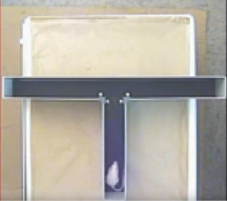
|

|
Running the RL-SNN Model
To fit the RL-SNN model described above, go to the exhibits/rl_snn
sub-folder (this step assumes that you have git cloned the model museum repo
code), and execute the RL-SNN’s simulation script from the command line as follows:
$ ./sim.sh
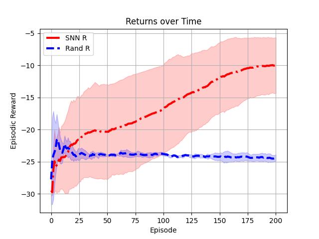
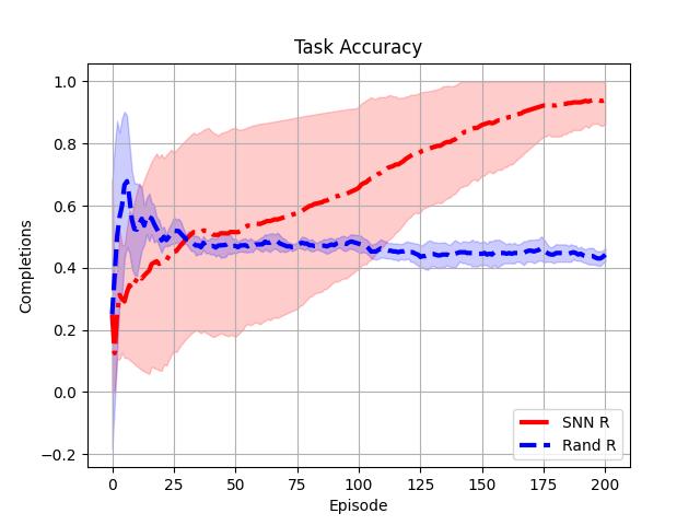
which will execute a simulation of the MSTDP-adapted SNN on the T-maze problem, specifically executing four uniquely-seeded trial runs (i.e., four different “rat agents”) and produce two plots, one containing a smoothened curve of episodic rewards over time and another containing a smoothened task accuracy curve (as in, did the rat reach the goal-state and obtain the food substance or not). You should obtain plots that look roughly like the two below.
|
|
Notice that we have provided a random agent baseline (i.e., uniform random selection of one of the four possible directions to move at each step in an episode) to contrast the SNN rat motor circuit’s performance with. As you may observe, the SNN circuit ultimately becomes conditioned to taking actions akin to the optimal policy – go North/up if it perceives itself (marked as a cross “+”) at the bottom of the T-maze and then go East/right once it has reached the top of the T of the T-maze and go right upon perception of the food item (goal state marked as an “X”).
The code has been configured to also produce a small video/GIF of the final episode episode200.gif, where the MSTDP
weight changes have been disabled and the agent must solely rely on its memory of the uncovered policy to get to the
goal state.
Some Important Limitations
While the above MSTDP-ET-driven motor circuit model is useful and provides a simple model of operant conditioning in the context of a very simple maze navigation task, it is important to identify the assumptions/limitations of the above setup. Some important limitations or simplifications that have been made to obtain a consistently working RL-SNN model:
As mentioned earlier, the sensory input contains a global view of the maze navigation problem, i.e., a 2D birds-eye view of the agent, its goal (the food substance), and its environment. More realistic, but far more difficult versions of this problem would need to consider an ego-centric view (making the problem a partially observable Markov decision process), a more realistic 3D representation of the environment, as well as more complex maze sizes and shapes for the agent/rat model to navigate.
The reward is only delayed with respect to the agent’s stimulus processing window, meaning that the agent essentially receives a dopamine signal after an action is taken. If we ignore the SNN’s stimulus processing time between video frames of the actual navigation problem, we can view our agent above as tackling what is known in reinforcement learning as the dense reward problem. A far more complex, yet more cognitively realistic, version of the problem is to administer a sparse reward, i.e., the rat motor circuit only receives a useful dopamine/reward stimulus at the end of an episode as opposed to after each action. The above MSTDP-ET model would struggle to solve the sparse reward problem and more sophisticated models would be required in order to achieve successful outcomes, i.e., appealing to models of memory/cognitive maps, more intelligent forms of exploration, etc.
The SNN circuit itself only permits plastic synapses in its control layer (i.e., the synaptic connections between the second layer and third output/control layer). The bottom layer is non-plastic and fixed, meaning that the agent model is dependent on the quality of the random initialization of the input-to-hidden encoding layer. The input-to-hidden synapses could be adapted with STDP (or MSTDP); however, the agent will not always successfully and stably converge to a consistent policy as the encoding layer’s effectiveness is highly dependent on how much of the environment the agent initially sees/explores (if the agent gets “stuck” at any point, STDP will tend to fill up the bottom layer receptive fields with redundant information and make it more difficult for the control layer to learn the consequences of taking different actions).
References
[1] Chevtchenko, Sérgio F., and Teresa B. Ludermir. “Learning from sparse and delayed rewards with a multilayer
spiking neural network.” 2020 International Joint Conference on Neural Networks (IJCNN). IEEE, 2020.
[2] Diehl, Peter U., and Matthew Cook. “Unsupervised learning of digit recognition using spike-timing-dependent
plasticity.” Frontiers in computational neuroscience 9 (2015): 99.