Sparse Coding and Iterative Thresholding (Olshausen & Field; 1996)

In this exhibit, we create, simulate, and visualize the internally acquired filters/atoms of variants of a sparse coding system based on the classical model proposed by (Olshausen & Field, 1996) [1]. After going through this demonstration, you will:

1. Learn how to build a 2-layer sparse coding model of natural image patterns, using the original dataset used in [1].

2. Visualize the acquired filters of the learned dictionary models and examine the results of imposing a kurtotic prior as well as a thresholding function over latent codes.

The model code for this exhibit can be found here.

Note: You will need to unzip the data arrays in exhibits/data/natural_scenes.zip to the folder exhibits/data/ to work through this exhibit.

On Dictionary Learning

Dictionary learning poses a very interesting question for statistical learning: can we extract “feature detectors” from a given database (or collection of patterns) such that only a few of these detectors play a role in reconstructing any given, original pattern/data point? The aim of dictionary learning is to acquire or learn a matrix, also called the “dictionary”, which is meant to contain “atoms” or basic elements inside this dictionary (such as simple fundamental features such as the basic strokes/curves/edges that compose handwritten digits or characters). Several atoms (or rows of this matrix) inside the dictionary can then be linearly combined to reconstruct a given input signal or pattern. A sparse dictionary model is able to reconstruct input patterns with as few of these atoms as possible. Typical sparse dictionary or coding models work with an over-complete spanning set, or, in other words, a latent dimensionality (which one could think of as the number of neurons in a single latent state node of an ngc-learn system) that is greater than the dimensionality of the input itself.

From a neurobiological standpoint, sparse coding emulates a fundamental property of neural populations – the activities among a neural population are sparse where, within a period of time, the number of total active neurons (those that are firing) is smaller than the total number of neurons in the population itself. When sensory inputs are encoded within this population, different subsets (which might overlap) of neurons activate to represent different inputs (one way to view this is that they “fight” or compete for the right to activate in response to different stimuli). Classically, it was shown in [1] that a sparse coding model trained on natural image patches learned within its dictionary non-orthogonal filters that resembled receptive fields of simple-cells (found in the visual cortex).

Constructing a Sparse Coding System

To build a sparse coding model, we can manually craft a model using ngc-learn’s nodes-and-cables system. First, we specify the underlying generative model we aim to emulate. Formally, we seek to optimize a set of latent codes according to the following differential equation:

\[ \tau_m \frac{\partial \mathbf{z}_t}{\partial t} = \big(\mathbf{W}^T \cdot \mathbf{e}(t) \big) + \lambda \Omega\big(\mathbf{z}(t)\big) \]

where the above is also referred to as the E-step (since the optimization carried out for most sparse coding models is done within the framework of expectation-maximization – E-step refers to updates to the latent variables whereas M-step refers to updates to synaptic/dictionary parameters) and \(\tau_m\) is the latent code time constant and the error neurons \(\mathbf{e}(t)\) at the sensory input layer made at time \(t\) are specified as:

\[ \mathbf{e}(t) = -\big(\mathbf{o}_t - (\mathbf{W} \cdot \mathbf{z}(t)) \big) \]

where we see that we aim to learn a two-layer generative system that specifically imposes a prior distribution p(z) over the latent feature detectors (via the constraint function \( \Omega\big(\mathbf{z}(t)\big) \) ) that we hope to extract in node z. Note that this two-layer model (or single latent-variable layer model) could either be the linear generative model from [1] or one similar to the model learned through ISTA [2] if a (soft) thresholding function is used instead.

Furthermore, the synaptic weight updates (the M-step) to our sparse coding model generally adhere to the following differential equation:

\[ \tau_m \frac{\partial \mathbf{W}}{\partial t} = -\mathbf{W} + \big(\mathbf{e}(t) \cdot (\mathbf{z}(t))^T \big) \]

Constructing the above system for (Olshausen & Field, 1996) is done, much like we do in the SparseCoding agent constructor in the model museum exhibit code, as follows:

from ngclearn.utils.io_utils import makedir
from ngclearn.utils.viz.synapse_plot import visualize
from jax import numpy as jnp, random, jit
from ngclearn import Context, MethodProcess, JointProcess
from ngclearn.components.neurons.graded.rateCell import RateCell
from ngclearn.components.synapses.denseSynapse import DenseSynapse
from ngclearn.components.synapses.hebbian.hebbianSynapse import HebbianSynapse
from ngclearn.components.neurons.graded.gaussianErrorCell import GaussianErrorCell as ErrorCell
from ngclearn.utils.model_utils import normalize_matrix
from ngclearn.utils.distribution_generator import DistributionGenerator as dist

in_dim =  # ... dimension of patch data ...
hid_dim =  # ... number of atoms in the dictionary matrix
dt = 1.  # ms
T = 300  # ms # (OR) number of E-steps to take during inference
# ---- build a sparse coding linear generative model with a Cauchy prior ----
with Context("Circuit") as circuit:
    z1 = RateCell(
        "z1", n_units=hid_dim, tau_m=20, act_fx="identity", prior=("cauchy", 0.14), integration_type="euler"
    )
    e0 = ErrorCell("e0", n_units=in_dim)
    W1 = HebbianSynapse(
        "W1", shape=(hid_dim, in_dim), eta=1e-2, weight_init=dist.fan_in_gaussian(), bias_init=None, w_bound=0., optim_type="sgd", sign_value=-1.
    )
    E1 = DenseSynapse( ## E1 = (W1)^T
        "E1", shape=(in_dim, hid_dim), weight_init=dist.uniform(-0.2, 0.2), 
        resist_scale=1.
    )
    E1.weights.set(W1.weights.get().T)

    ## wire z1.zF to e0.mu via W1
    z1.zF >> W1.inputs
    W1.outputs >> e0.mu
    ## wire e0.dmu back up to z1.j via E1 (for E-step)
    e0.dmu >> E1.inputs
    E1.outputs >> z1.j
    
    ## Setup W1 for its 2-factor Hebbian update (for M-step)
    z1.zF >> W1.pre
    e0.dmu >> W1.post

    ## Inference process
    advance = (MethodProcess(name="advance")
               >> W1.advance_state
               >> E1.advance_state
               >> z1.advance_state
               >> e0.advance_state)
    ## Reset-to-baseline process
    reset = (MethodProcess(name="reset")
             >> W1.reset
             >> E1.reset
             >> z1.reset
             >> e0.reset)
    ## Learning process
    evolve = (MethodProcess(name="evolve")
              >> W1.evolve)

There is one important co-routine we also need to make sure we include for our sparse coding circuit that needs to happen after each update to the synapses – synaptic weight normalization. Specifically, we want to normalize the Euclidean norm of the columns of the dictionary matrix to be equal to a value of one.

This is a particularly important constraint to apply to sparse coding models as this prevents the trivial solution of simply growing out the magnitude of the dictionary synapses to solve the underlying constrained optimization problem (and, in general, constraining the rows or columns of generative models helps to facilitate a more stable training process). This norm constraint can be simply written as below:

def norm():
    W1.weights.set(normalize_matrix(W1.weights.get(), 1., order=2, axis=1))

To build the version of our model (the ISTA model) using a thresholding function, instead of using a factorial prior over the latents, we can write the following:

# ---- build a sparse coding generative model w/ a thresholding function ----
with Context("Circuit") as circuit:
    z1 = RateCell(
        "z1", n_units=hid_dim, tau_m=20, act_fx="identity", threshold=("soft_threshold", 5e-3), integration_type="euler"
    )
    e0 = ErrorCell("e0", n_units=in_dim)
    W1 = HebbianSynapse(
        "W1", shape=(hid_dim, in_dim), eta=1e-2, weight_init=dist.fan_in_gaussian(), bias_init=None, w_bound=0., optim_type="sgd", sign_value=-1.
    )
    E1 = DenseSynapse(
        "E1", shape=(in_dim, hid_dim), weight_init=dist.uniform(-0.2, 0.2), 
        resist_scale=1.
    )
    E1.weights.set(W1.weights.get().T)
    ## ...rest of the code is the same as the Cauchy prior model...

Note that the above two models are built and configured for you in the Model Museum, in the museum/exhibits/olshausen_sc/sparse_coding.py agent constructor, which internally implements the model contexts depicted above as well as the necessary task-specific functions needed to reproduce the correct experimental setup (these get compiled in the constructor’s dynamic() method. For both the Cauchy prior model of [1] and the iterative thresholding model of [2], we track, in the training script train_patch_sc.py, various dictionary synaptic statistics and a measurement of the model reconstruction loss. The reconstruction loss is a key part of the objective that both models optimize, i.e., both SC models effectively optimize an energy function that is a sum of its reconstruction error of its sensory input and the sparsity of its single latent state layer z1).

Learning Latent Feature Detectors

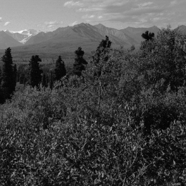
We will now simulate the learning of feature detectors using the two sparse coding models specified above. The code provided in train_patch_sc.py will execute a simulation of the above two models on the natural images found in exhibits/data/natural_scenes.zip), which is a dataset composed of several images of the American Northwest.

First, navigate to the exhibits/ directory to access the example/demonstration code and further enter the exhibits/data/ sub-folder. Unzip the file natural_scenes.zip to create one more sub-folder that contains two numpy arrays, the first labeled natural_scenes/raw_dataX.npy and another labeled as natural_scenes/dataX.npy. The first one contains the original, 512 x 512 raw pixel image arrays (flattened) while the second contains the pre-processed, whitened/normalized (and flattened) image data arrays (these are the pre-processed image patterns used in [1]). You will, in this demonstration, only be working with natural_scenes/dataX.npy. Two (raw) images sampled from the original dataset (raw_dataX.npy) are shown below:

With the data unpacked and ready, we can now run the training process in the model exhibit by either executing its Python simulation script like so:

$ python train_patch_sc.py --dataX="$DATA_DIR/dataX.npy" \
                           --n_iter=200 --model_type="sc_cauchy"

or simply running the convenience Bash script $ ./sim.sh (which cleans up the model experimental output folder each time you call the training script in order to reduce memory clutter on your system). Running either the Python or Bash script will then train a sparse coding model with a Cauchy prior on 16 x 16 pixel patches from the natural image dataset in [1].[1] After the simulation terminates, i.e., once 200 iterations/passes through the data have been made, you will notice in the exp/filters/ sub-directory a visual plot of your trained model’s filters which should look like the one below:

If you modify either the Bash script or Python script call to use with a different model argument like so:

$ python train_patch_sc.py --dataX="$DATA_DIR/dataX.npy" \
                           --n_iter=200 --model_type="sc_ista"

you will now train your sparse coding using a latent soft-thresholding function (emulating ISTA). After this simulated training process ends, you should see in your exp/filters/ sub-directory a filter plot like the one below:

The filter plots, notably, visually indicate that the dictionary atoms in both sparse coding systems learned to function as edge detectors, each tuned to a particular position, orientation, and frequency. These learned feature detectors, as discussed in [1], appear to behave similar to the primary visual area (V1) neurons of the cerebral cortex in the brain. In the end, even though the edge detectors learned by both our models qualitatively appear to be similar, we should note that the latent codes (when inferring them given sensory input) for the model that used the thresholding function will ultimately sparser (given the direct clamping to zero values it imposes mathematically).
Furthermore, the filters for the model with thresholding appear to smoother and with fewer occurrences of less-than-useful slots than the Cauchy model (or filters that did not appear to extract any particularly interpretable features).

Computing Hardware Note:

This tutorial was tested and run on an Ubuntu 22.04.2 LTS operating system using an NVIDIA GeForce RTX 2070 GPU with CUDA Version: 12.1 (Driver Version: 530.41.03). Note that the times reported in any tutorial screenshot/console snippets were produced on this system.

References

[1] Olshausen, B., Field, D. Emergence of simple-cell receptive field properties by learning a sparse code for natural images. Nature 381, 607–609 (1996).
[2] Daubechies, Ingrid, Michel Defrise, and Christine De Mol. “An iterative thresholding algorithm for linear inverse problems with a sparsity constraint.” Communications on Pure and Applied Mathematics: A Journal Issued by the Courant Institute of Mathematical Sciences 57.11 (2004): 1413-1457.

---

[1]

Ultimately, the sparse coding training process consists of the following steps: 1) sample a random image from the image design matrix inside of the in-built ngc-learn DataLoader, 2) generate a number of patches equal to num_patches = 250 (which we have also hard-coded into train_patch_sc.py), and 3) feed this mini-batch of image patches to the sparse coding model to facilitate an expectation-maximization (E-M) step, where we take T=300 E-steps followed by one single M-step and a norm constraint application.