The Diehl and Cook Spiking Neuronal Network (Diehl & Cook; 2015)

In this exhibit, we will see how a spiking neural network model that adapts its synaptic efficacies via spike-timing-dependent plasticity can be created. This exhibit model effectively reproduces some of the results reported (Diehl & Cook, 2015) [1]. The model code for this exhibit can be found here.

Note: You will need to unzip the MNIST arrays in exhibits/data/mnist.zip to the folder exhibits/data/ to work through this exhibit/walkthrough.

The Diehl and Cook Spiking Network (DC-SNN)

The Diehl and Cook spiking neural network [1] (which we abbreviate to “DC-SNN”) is an important model of spiking neuronal dynamics that crucially demonstrated effective unsupervised learning on MNIST digit patterns. Furthermore, it is a rather useful model for getting a handle on the interaction between explicit excitatory neurons and inhibitory neurons (where cell in both populations/groups are leaky integrators). In ngc-learn, constructing a DC-SNN is straightforward using its in-built leaky integrator, the LIFCell, which is what this model exhibit does for you in the DC_SNN model constructor.[1] The DC-SNN model in this exhibit also makes use of one of ngc-learn’s in-built spike-timing-dependent plasticity synapses in order to recover one of the ways that [1] adapted its synaptic strengths.

Neuronal Dynamics

The DC-SNN is effectively made up of three layers:

1. a sensory input layer made up of Poisson encoding neuronal cells (which are configured in the exhibit model to fire spikes at a maximal frequency of 63.75 Hertz as in [1]);

2. one hidden layer of excitatory leaky integrate-and-fire (LIF) cells; and,

3. one (laterally-wired) hidden layer of inhibitory LIF cells.

The sensory input layer connects to excitatory layer with a synaptic cable W1 (\(\mathbf{W}^1_t\)) – which will be adapted with (traced-based) spike-timing-dependent plasticity as we will describe in the next section. The excitatory layer of the model connects to the inhibitory layer with a fixed identity synaptic cable (ensuring that all excitatory neurons map one-to-one to the inhibitory ones) while the inhibitory layers are connected to the excitatory layer via a fixed, negatively scaled hollow synaptic cable.

The dynamics on the structure described above result in a form of sensory input-driven excitatory LIF dynamics that are recurrently inhibited by the laterally-wired inhibitory LIF cells (or LIFs). Formally, the excitatory and inhibitory neurons in the DC-SNN exhibit both adhere to the following ordinary differential equation (ODE):

\[ \tau_m \frac{\partial \mathbf{v}_t}{\partial t} = (v_{rest} -\mathbf{v}_t + R \mathbf{j}_t) \odot \mathbf{m}_{rfr} \]

where \(v_{rest}\) is the resting potential (in milliVolts, mV) and \(\mathbf{m}_{rfr}\) is a binary mask where any element is zero if the neuronal cell is in its refractory period (meaning that it will be clamped to its resting/reset potential for so many milliseconds). Note that \(\odot\) denotes an elementwise multiplication (Hadamard product) and \(\cdot\) denotes a matrix-vector multiplication. Spikes are emitted from any cell within \(\mathbf{v}_t\) according to the following piecewise function:

\[\begin{split} \mathbf{s}_{t, i} = \begin{cases} 1 & \mathbf{v}_{t, i} > \theta_{t, i} \\ 0 & \mbox{otherwise.} \end{cases} \end{split}\]

and any neuron that breached its threshold value and emitted a (binary) spike is immediately set to its \(v_{reset}\) potential (mV); note that \(v_{reset}\) might not be the same as the \(v_{rest}\). \(\theta_t\) contains all of the current voltage threshold values (and is the same shape as \(\mathbf{v}_t\)). In ngc-learn, the LIFCell component also evolves \(\theta_t\) to according its own set of dynamics as follows:

\[\begin{split} \tau_\delta \frac{\partial \delta}{\partial t} &= -\delta + \alpha \mathbf{s}_t \\ \theta_t &= \theta_{base} + \delta \end{split}\]

where \(\delta\) is a “homeostatic variable” that essentially increments (any dimension \(i\)) by a small constant amount every time a particular cell \(i\) emits a spike (setting \(\tau_\delta = 0\) turns off the threshold dynamics). Note that the second equation above implies that \(\theta_t\) does not evolve its base threshold value (\(\theta_{base}\)), it is simply re-computed as a sum of its base value and the current value of the evolved homeostatic variable. With the above knowledge, we can now effectively recreate the setup of [1] by using a value greater than zero for \(\tau_\delta\) for the excitatory LIFs and a value of zero (for \(\tau_\delta\)) for the inhibitory ones.

Finally, the last key item to specify is how the electrical current is produced along synapses for the excitatory and inhibitory neurons. For the excitatory LIFs, the electrical currents can be produced either as their own evolving ODE (as in [1]) or simplified to pointwise currents[2]. This entails, in the DC_SNN exhibit class, the following (synaptic) wiring scheme:

\[\begin{split} \mathbf{j}^e_t &= \mathbf{W}^1_t \cdot \mathbf{s}^{inp}_t - \big((1 - \mathbf{I}) \odot \mathbf{W}^{ie}\big) \cdot \mathbf{s}^i_t \\ \mathbf{j}^i_t &= \big(\mathbf{I} \odot \mathbf{W}^{ei}\big) \cdot \mathbf{s}^e_t \end{split}\]

where we denote an excitatory spike vector as \(\mathbf{s}^e_t\), an inhibitory spike vector as \(\mathbf{s}^i_t\), and an input (Poisson) spike vector as \(\mathbf{s}^{inp}_t\). As mentioned earlier, \(\mathbf{W}^1_t\) is the input-to-excitatory synaptic cable while \(\mathbf{W}^{ei}\) is the excitatory-to-inhibitory synaptic cable \(\mathbf{W}^{ie}\) is the inhibitory-to-excitatory synaptic cable; the subscript \(t\) has been dropped for these last two cables (\(\mathbf{W}^{ei}\) and \(\mathbf{W}^{ie}\)) because they are held fixed to constant values [1]. Ultimately, the inhibitory neurons will emit spikes once enough voltage has been built up as they receive enough electrical current driven by the excitatory neurons – once the inhibitory neurons fire, they will laterally inhibit/suppress the activities of other excitatory cells (besides the one they receive electrical current directly from). This type/pattern of cross-layer inhibition will induce a form of “lateral competition” in the dynamics of the excitatory neural units, where few units specialize represent particular types/kinds of input patterns (these competitive dynamics are important for effective adaptation of synapses via STDP).

The spiking neural system that the above specifies will engage in a form of unsupervised representation learning, simply resulting in sparse spike-train patterns that correlate with different input digit patterns sampled from the MNIST database. The figure below depicts the DC-SNN architecture, particularly showing the case where only one out of the population of excitatory neuronal cells gets triggered and drives its corresponding inhibitory cell which transmits back/laterally suppression signals to all but the triggered excitatory neuron.

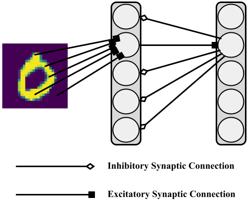
All that remains is to specify the synaptic plasticity dynamics (learning) for the DC-SNN, which we do next.

Spike-Timing-Dependent Plasticity (STDP)

Adaptation/plasticity in our DC-SNN is rather simple – in this model exhibit, a form of STDP is used to adapt the synaptic weight values (specifically, it is trace-based STDP), which models a form of long-term depression (LTD) and long-term potentiation (LTP) to adjust synapses according to a Hebbian-like rule as follows (in matrix-vector format):

\[ \tau_{syn} \frac{\partial \mathbf{W}^1_t}{\partial t} = A_{+} \Big(\mathbf{s}^e_t \cdot (\mathbf{z}^{inp}_t - z_{tar})^T\Big) - A_{-} \Big(\mathbf{z}^e_t \cdot (\mathbf{s}^{inp}_t)^T\Big) \]

where we see that LTP is modeled by the first term (to the left of the minus sign) – a product of the (excitatory) post-synaptic spike(s)/event(s) that might have occurred at time \(t\) and the value of the pre-synaptic trace[3] at the occurrence of spikes at \(t\) – and that LTD is modeled by the second term (to the right of the minus sign) – a product of the (excitatory) post-synaptic trace at time \(t\) and the pre-synaptic spike(s)/event(s) that might have happened at \(t\). \(A_{+}\) is the scaling factor controlling how much LTP is applied to a synaptic update and \(A_{-}\) controls how LTD would be applied to the update. \(()^T\) denotes the matrix/vector transpose while \(z_{tar}\) is a pre-synaptic trace target value and set to \(0\) in the default configuration of the DC-SNN (in [1], this value was used in one of the variants of STDP investigated; if it is set to be \(> 0\), then rarely spiking neurons in the input layer will be effectively disconnected from the excitatory layer, effectively fading away to zero). Roughly speaking, the above in-built STDP rule in ngc-learn effectively applies the idea that, for a pre-synaptic neurons \(i\) in the input layer and a post-synaptic neuron \(j\) in the excitatory layer (in our DC-SNN model), we increase the efficacy value of the synapse \(W^1_{ij}\) (that connects them; that integers \(i\) and \(j\) retrieve a specific scalar within our synaptic cable \(\mathbf{W}^1_t\)) if neuron \(j\) spikes after neuron \(i\) and we decrease the efficacy value \(W^1_{ij}\) if neuron \(i\) spikes before neuron \(j\).

There a few other small details beyond the trace-based STDP rule that is applied to this model, such as a synaptic rescaling step applied at particular steps in time (as was done in [1]). Notes on these minor extra mechanisms can be found in the DC-SNN’s README.

Running the DC-SNN Model

To fit the DC-SNN model described above, go to the exhibits/diehl_cook_snn sub-folder (this step assumes that you have git cloned the model museum repo code), and execute the DC-SNN’s simulation script from the command line as follows:

$ ./sim.sh

which will execute a training process using an experimental configuration very similar to (Diehl & Cook, 2015). Note that since STDP-adaptation of synapses is unsupervised, there really is no known objective function or cost functional for us to track (this is an ongoing topic of research in the fields of brain-inspired computing and computational neuroscience); as a result, the train_dcsnn.py script prints out every 500 digits processed some synaptic statistics that demonstrate learning is occurring.[4] After your model finishes training you should see output similar to the one below:

------------------------------------
 Trial.sim_time = 0.7072688111994001 h  (2546.1677203178406 sec)

To use your saved model and examine its performance on the MNIST test-set, you can execute the evaluation script like so:

$ python analyze_dcsnn.py --dataX=../../data/mnist/testX.npy --sample_idx=0

while will produce a visualization of your DC-SNN’s receptive fields (the synaptic values inside of W1) in the /exp/filters/ sub-directory:

After only seeing 10,000 digit patterns (online), the DC-SNN already seems to have acquired representative synaptic “templates” or receptive fields that correspond to digits across the class categories in the MNIST database (at least one template for each of the ten unique classes).

Furthermore, running the analyze_dcsnn.py also produces a useful sample raster plot of the DC-SNN’s excitatory neurons for the default sampled test digit (index 99) in the /exp/raster/ sub-directory. You should see a raster plot much like
the one below:

As observed (we have overlaid pink box zoom-ins to emphasize the locations of the spike ticks), due to the competitive dynamics of this model, the spike train for this trained model end up being very sparse (and thus quite friendly for neuromorphic platforms, where a hard zero means no computation needs to be carried out, thus avoiding propagating zero values along synapses in multi-layer neuronal models).

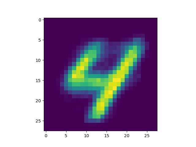
One final item you will notice produced by analyze_dcsnn.py are two small images in /exp/, i.e., digit0.png and syn<NUMBER>_digit0.png – these particular images are created due to your choice of sample_idx (where you should pick an integer between 0 and one less than the maximum number of images in the dataset you are studying ). For instance, you might get the following two images (if you use the same synaptic values as we obtained from training):

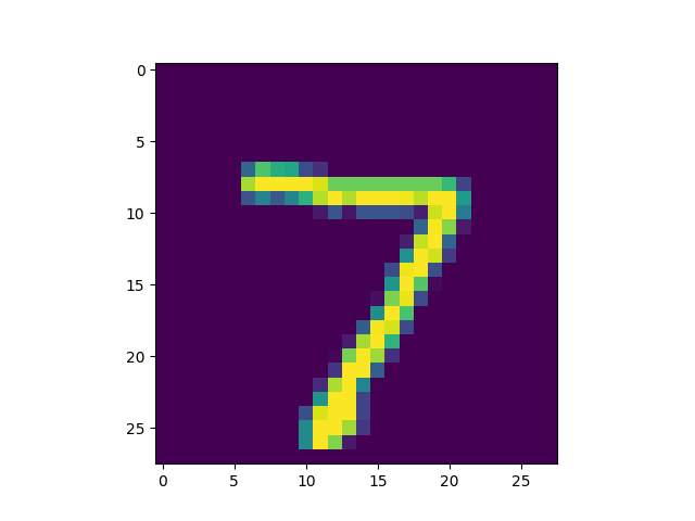
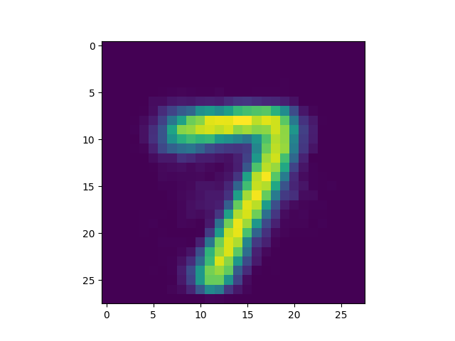
In the images above, we observe that synaptic slice (or receptive field) number 58 (i.e., <NUMBER> = 58) was matched by model to image pattern 0.

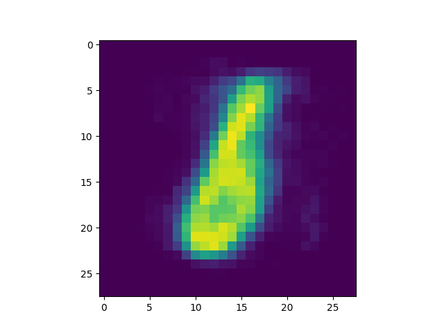
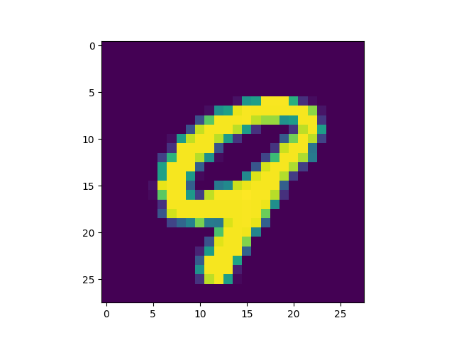
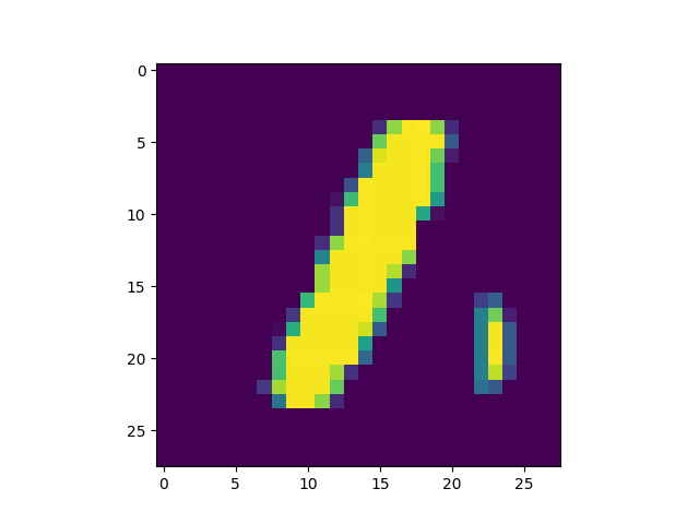
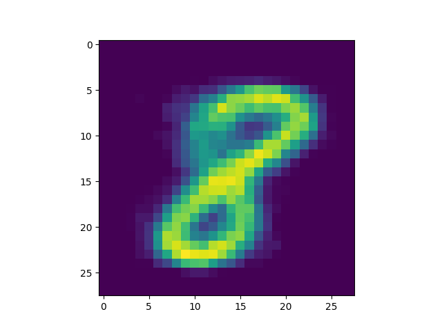
Changing the sample_idx argument to the analyze_dcsnn.py allows you, in this model exhibit code, to query different image patterns against your trained DC-SNN model (like it’s a “neural lookup table”). Studying our trained model from the exhibit code, (a zip containing the synapses our simulation produced is included[5]) we got some interesting successful matches:

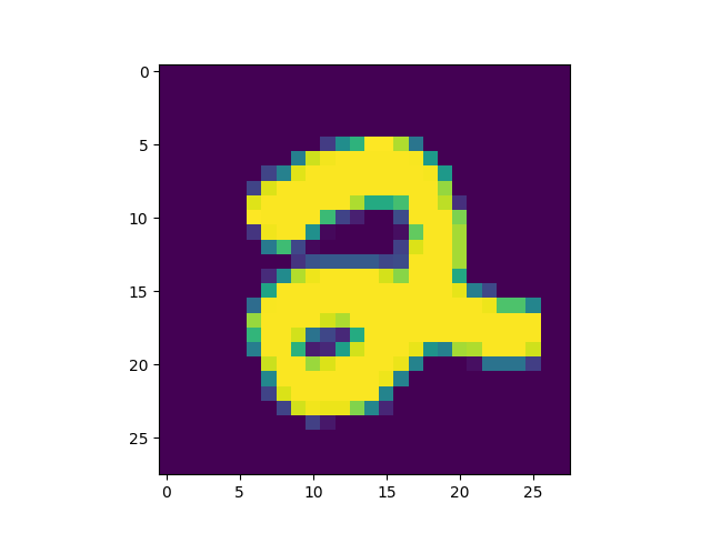
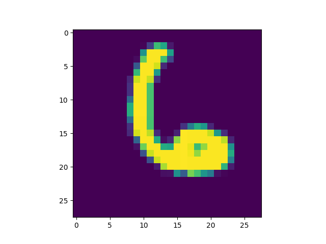
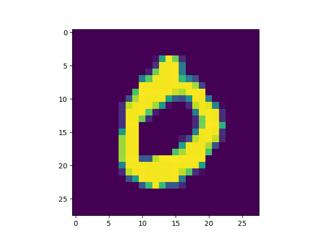
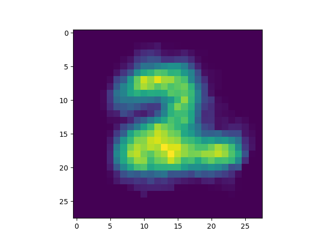
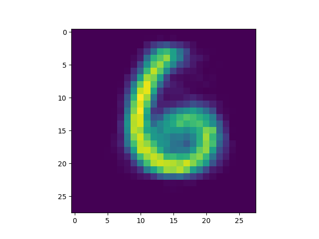
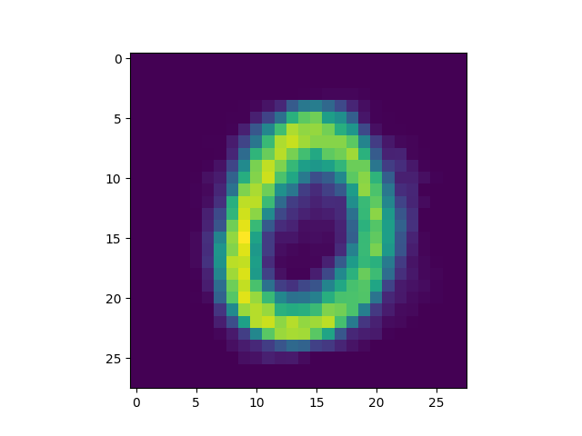
as well as some interesting failures:

Obviously, the DC-SNN we trained is rather small (only 100 neurons in the exhibit file’s default configuration) and was only trained online on the first 10000 digits. Different results would be obtained if more digit patterns were used and more excitatory neurons were utilized.

Computing Hardware Note:

This tutorial was tested and run on an Ubuntu 22.04.2 LTS operating system using an NVIDIA GeForce RTX 2070 GPU with CUDA Version: 12.1 (Driver Version: 530.41.03). Note that the times reported in any tutorial screenshot/console snippets were produced on this system.

References

[1] Diehl, Peter U., and Matthew Cook. “Unsupervised learning of digit recognition using spike-timing-dependent plasticity.” Frontiers in computational neuroscience 9 (2015): 99.

---

[1]

Note that the LIFCell is not the same as ngc-learn’s sLIFCell, which is a particular cell that simplifies the spiking dynamics greatly and is not meant to operate in the negative milliVolt range like the LIFCell does.

[2]

While both forms of modeling electrical current are easily doable in NGC-Learn, the DC_SNN exhibit model opts for the second approach for simplicity and additional simulation speed.

[3]

Trace components have also been used in the DC_SNN exhibit model, specifically those built with the variable trace component. Note that the variable trace effectively applies a low-pass filter iteratively to the spikes produced by a spike train.

[4]

In the NAC group’s experience, observing the mean and Frobenius norm of synaptic values can be a useful starting point for determining unhealthy behavior or some degenerate cases in the context of spiking neural network credit assignment.

[5]

To load in the exact synaptic efficacies we obtained to get the images above, you can unzip the folder dcsnn_syn.zip, which contains all of the model’s numpy array values, and simply copy all of the compressed numpy arrays into your exp/snn_stdp/custom/ folder, which is where ngc-learn/ngc-sim-lib look for pre-trained value arrays when loading in a previously constructed model. Once you do this, running analyze_dcsnn.py with the same arguments as above should produce plots/images much like those in this walkthrough.