Lecture 4C: Spike-Timing-Dependent Plasticity
In the context of spiking neuronal networks, one of the most important forms of adaptation that is often simulated is that of spike-timing-dependent plasticity (STDP). In this lesson, we will setup and use one of ngc-learn’s standard in-built STDP-based components, visualizing the changes in synaptic efficacy that it produces in the context of pre-synaptic and post-synaptic variable traces.
Probing Spike-Timing-Dependent Plasticity
Go ahead and make a new folder for this study and create a Python script, i.e., run_trstdp.py, to write your code for this part of the tutorial.
Now let’s set up the model for this lesson’s simulation and construct a 3-component system made up of two variable traces (VarTrace) connected by one single synapse that is capable of producing changes in connection strength in accordance with STDP, specifically with a form of the update rule known as trace-based STDP. Note that the trace components do not really do anything meaningful unless they receive some input. Therefore, we will provide carefully controlled input spike values in order to control their behavior in order to see how STDP responds to the relative temporal ordering of a pre- and post-synaptic spike, where the timing of the spikes is approximated by the corresponding pre- and post-synaptic traces (which decay exponentially with time in the absence of input).
Writing the above 3-component system can be done in the following manner:
from jax import numpy as jnp, random, jit

from ngclearn import Context, MethodProcess
## import model-specific mechanisms
from ngclearn.components.other.varTrace import VarTrace
from ngclearn.components.synapses.hebbian.traceSTDPSynapse import TraceSTDPSynapse
from ngclearn.utils.distribution_generator import DistributionGenerator

## create seeding keys (JAX-style)
dkey = random.PRNGKey(231)
dkey, *subkeys = random.split(dkey, 2)

dt = 1.  # ms # integration time constant
T_max = 100  ## number time steps to simulate

with Context("Model") as model:
    tr0 = VarTrace("tr0", n_units=1, tau_tr=8., a_delta=1.)
    tr1 = VarTrace("tr1", n_units=1, tau_tr=8., a_delta=1.)
    W = TraceSTDPSynapse(
        "W1", shape=(1, 1), eta=0., A_plus=1., A_minus=0.8,
        weight_init=DistributionGenerator.uniform(low=0.0, high=0.3), key=subkeys[0]
    )

    # wire only relevant compartments to synaptic cable W for demo purposes
    tr0.trace >> W.preTrace
    # self.z0.outputs >> self.W1.preSpike ## we disable this as we will manually
    ##                                       insert a binary value (for a spike) in this tutorial
    tr1.trace >> W.postTrace
    # self.z1e.s >> self.W1.postSpike ## we disable this as we will manually
    ##                                   insert a binary value (for a spike) in this tutorial

    evolve_synapse = (MethodProcess("evolve")
                      >> W.evolve)

    advance_traces = (MethodProcess("advance")
                      >> tr0.advance_state
                      >> tr1.advance_state
                      >> W.advance_state)

    reset = (MethodProcess("reset")
             >> tr0.reset
             >> tr1.reset
             >> W.reset)

## set up some utility functions for the model context
def clamp_synapse(pre_spk, post_spk):
    W.preSpike.set(pre_spk)
    W.postSpike.set(post_spk)

def clamp_traces(pre_spk, post_spk):
    tr0.inputs.set(pre_spk)
    tr1.inputs.set(post_spk)
With our carefully constructed STDP-adapted model above, we can then simulate the changes to synaptic efficacy that it would produce as a function of the distance between and order between a pre- and a post-synaptic binary spike. Notice that in the above model, we have set the global learning rate eta to zero, which will prevent the TraceSTDPSynapse from actually adjusting its internal matrix of synaptic weight values using the updates produced by STDP – this means our synapses are held fixed throughout this particular demonstration. Our goal is to produce an approximation of the theoretical synaptic strength adjustment curve dictated by STDP; this can be done using the code below:
t_values = []
dW_vals = []
## run traces for T_max
_pre_trig = jnp.zeros((1,1))
_post_trig = jnp.zeros((1,1))
ts = -int(T_max/2) * 1.
for i in range(T_max+1):
pre_spk = jnp.zeros((1,1))
post_spk = jnp.zeros((1,1))
if i == int(T_max/2): ## switch to post-spike case
pre_spk = jnp.ones((1,1))
post_spk = jnp.zeros((1,1))
_pre_trig = jnp.zeros((1,1))
_post_trig = jnp.ones((1,1))
ts = 0.
elif i == 0: ## switch to pre-spike case
pre_spk = jnp.zeros((1,1))
post_spk = jnp.ones((1,1))
_pre_trig = jnp.ones((1,1))
_post_trig = jnp.zeros((1,1))
ts = 0.
clamp_traces(pre_spk, post_spk)
advance_traces.run(t=dt * i, dt=dt)
## get STDP update
clamp_synapse(_pre_trig, _post_trig)
evolve_synapse.run(t=dt * i, dt=dt)
dW = W.dWeights.get()
dW_vals.append(dW)
if i >= int(T_max/2):
t_values.append(ts)
ts += dt
else:
t_values.append(ts)
ts -= dt
dW_vals = jnp.squeeze(jnp.asarray(dW_vals))
import matplotlib #.pyplot as plt
matplotlib.use('Agg')
import matplotlib.pyplot as plt
cmap = plt.cm.jet
fig, ax = plt.subplots()
_tr0 = ax.plot(t_values, dW_vals, 'o', color='tab:red')
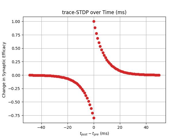
ax.set(xlabel='$t_{post} - t_{pre}$ (ms)', ylabel='Change in Synaptic Efficacy',
title='trace-STDP over Time (ms)')
ax.grid()
fig.savefig("stdp_curve.jpg")
which should produce a plot similar to the one in the left-hand side below:
|
|
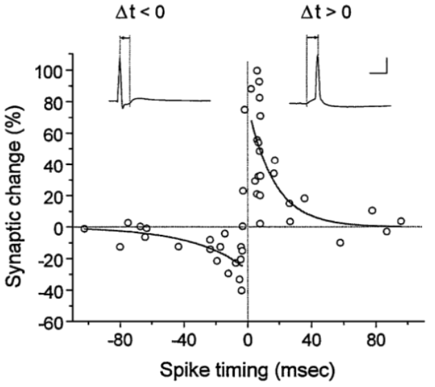
Notice that, for the above visual, we have also provided a marked-up image of the STDP experimental data produced and visualized in the classical work done by Bi and Poo in 1998 [1]. We remark that our approximate STDP synaptic change curve does not perfectly match/fit that of [1] perfectly by any means; however, it does capture the general trend and form of the long-term potentiation arc (the roughly negative exponential curve to the right-hand side of zero) and the long-term depression curve (the flipped exponential-like function to the left-hand side of zero). Ultimately, a synaptic component like the TraceSTDPSynapse can be quite useful for constructing spiking neural network architectures that learn in a biologically-plausible fashion given that this rule, as seen by the above simulation usage, solely depends on information that is locally available at the pre-synaptic neuron (its spike and a single trace that tracks its temporal spiking history) and the post-synaptic neuron (its own spike as well as a trace that tracks its spike history). Notably, traced-based STDP can be an effective way of adapting the synapses of biophysically more accurate computational models, such as those that balance excitatory and inhibitory pressures produced by laterally-wired populations of leaky integrator neurons, e.g., the Diehl and Cook spiking architecture that we study in more detail within the context of a model museum exhibit.
Other Forms of Spike-Timing-Dependent Plasticity
Finally, beyond trace-based STDP, there are other types of STDP in-built to ngc-learn, such as event-driven post-synaptic STDP (eventSTDPSynapse), which you can experiment with and use in your model building and simulation projects. You can learn more about these and other related biologically-plausible learning rules in the ngc-learn modeling API (specifically in the “Synapses” subsection page). Beyond this, the ngc-learn dev team is always busy behind the scenes constructing more standard computational neuroscience building blocks and synaptic plasticity rules; so keep an eye out for future incoming developments!
References
[1] Bi, Guo-qiang, and Mu-ming Poo. “Synaptic modifications in cultured hippocampal neurons: dependence on spike timing, synaptic strength, and postsynaptic cell type.” Journal of neuroscience 18.24 (1998).