Lecture 2E: The Adaptive Exponential Integrator Cell
In this tutorial, we will study a more complex variation of integrate-and-fire spiking dynamics in-built to ngc-learn, specifically the adaptive exponential (AdEx) integrate-and-fire biophysical neuronal cell model.
Using and Probing an AdEx Cell
Go ahead and make a new folder for this study and create a Python script,
i.e., run_adexcell.py, to write your code for this part of the tutorial.
Now let’s set up the controller for this lesson’s simulation and construct a single component system made up of an AdEx cell.
Instantiating the AdEx Neuronal Cell
Constructing/setting up a dynamical system made up of only a single AdEx cell amounts to the following:
from jax import numpy as jnp, random, jit
import numpy as np

from ngclearn import Context, MethodProcess
## import model-specific mechanisms
from ngclearn.components.neurons.spiking.adExCell import AdExCell

## create seeding keys (JAX-style)
dkey = random.PRNGKey(1234)
dkey, *subkeys = random.split(dkey, 6)

T = 10000  ## number of simulation steps to run
dt = 0.1  # ms ## compute integration time constant

## AdEx cell hyperparameters
v0 = -70.  ## initial membrane potential (for its reset condition)
w0 = 0.  ## initial recovery value (for its reset condition)

## create simple system with only one AdEx
with Context("Model") as model:
    cell = AdExCell(
        "z0", n_units=1, tau_m=15., resist_m=1., tau_w=400., v_sharpness=2.,
        intrinsic_mem_thr=-55., v_thr=5., v_rest=-72., v_reset=-75., a=0.1,
        b=0.75, v0=v0, w0=w0, integration_type="euler", key=subkeys[0]
    )
    ## create and compile core simulation commands
    advance_process = (MethodProcess("advance_proc")
                       >> cell.advance_state)
    reset_process = (MethodProcess("reset_proc")
                     >> cell.reset)

## set up non-compiled utility commands
def clamp(x):
    cell.j.set(x)
In effect, the AdEx two-dimensional differential equation system [1]-[2] offers
a more complex model of spiking cellular activation and deactivation
dynamics. Notably, the AdEx cell, like many of the more complex cells such
as the Izhikevich cell, is composed of a membrane potential v and a
recovery/adaptation variable w. The core voltage dynamics are a nonlinear
variation of those of the LIF cell and notably have some empirical support
from experimental neuroscience. More importantly, the AdEx model
can account for different neuronal firing patterns driven by injection of
constant electrical, such as bursting, initial bursting, and adaptation.
Formally, the core dynamics of the AdEx cell can be written out as follows:
where, furthermore, if a spike occurs, the recovery variable \(\mathbf{w}_t\) is reset according to \(\mathbf{w}_t \leftarrow \mathbf{w}_t + \mathbf{s}_t \odot (\mathbf{w}_t + b)\). \(a\) and \(b\) are factors that drive the recovery variable’s dynamics (scaling and shifting, respectively), \(R\) is the membrane resistance, \(\tau_m\) is the membrane time constant, and \(\tau_w\) is the recovery time constant. For the voltage dynamics, beyond the standard LIF coefficients, two new ones that shape the nonlinearity of the dynamics are \(s_V\) – the slope factor (this controls the sharpness of action potential initiation )– and \(v_{intr}\) – the intrinsic membrane threshold.
Simulating an AdEx Neuronal Cell
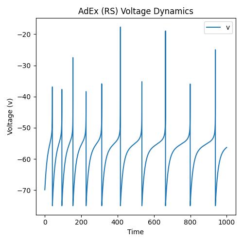
To see how the AdEx cell works, we can next write some code for visualizing how
the node’s membrane potential and coupled recovery variable evolve with time
(over a period of about 1000 milliseconds). We will inject an electrical
current j into the AdEx cell (specifically 19 amperes) and observe how the cell
produces its action potentials. Specifically, we create the simulation of this
constant current injection with the code below:
curr_in = []
mem_rec = []
recov_rec = []
spk_rec = []

i_app = 19. ## electrical current to inject into AdEx cell
data = jnp.asarray([[i_app]], dtype=jnp.float32)

time_span = []
reset_process.run()
t = 0.
for ts in range(T):
    x_t = data
    ## pass in t and dt and run step forward of simulation
    clamp(x_t)
    advance_process.run(t=t, dt=dt) # run one step of dynamics
    t = t + dt

    ## naively extract simple statistics at time ts and print them to I/O
    v = cell.v.get()
    w = cell.w.get()
    s = cell.s.get()
    curr_in.append(data)
    mem_rec.append(v)
    recov_rec.append(w)
    spk_rec.append(s)
    ## print stats to I/O (overriding previous print-outs to reduce clutter)
    print("\r {}: s {} ; v {} ; w {}".format(ts, s, v, w), end="")
    time_span.append((ts)*dt)
print()
and we can plot the neuron’s voltage v and recovery variable w dynamics with
the following:
import matplotlib #.pyplot as plt
matplotlib.use('Agg')
import matplotlib.pyplot as plt
cmap = plt.cm.jet
import matplotlib.patches as mpatches #used to write custom legends

## Post-process statistics (convert to arrays) and create plot
time_span = np.asarray(time_span)
curr_in = np.squeeze(np.asarray(curr_in))
mem_rec = np.squeeze(np.asarray(mem_rec))
recov_rec = np.squeeze(np.asarray(recov_rec))
spk_rec = np.squeeze(np.asarray(spk_rec))

# Plot the AdEx cell trajectory
n_plots = 1
fig, ax = plt.subplots(1, n_plots, figsize=(5*n_plots,5))
ax_ptr = ax
ax_ptr.set(
    xlabel='Time', ylabel='Voltage (v)', title="AdEx Voltage Dynamics"
)

v = ax_ptr.plot(time_span, mem_rec, color='C0')
ax_ptr.legend([v[0]],['v'])
plt.tight_layout()
plt.savefig("{0}".format("adex_v_plot.jpg"))

fig, ax = plt.subplots(1, n_plots, figsize=(5*n_plots,5))
ax_ptr = ax
ax_ptr.set(
    xlabel='Time', ylabel='Recovery (w)', title="AdEx Recovery Dynamics"
)
w = ax_ptr.plot(time_span, recov_rec, color='C1', alpha=.5)
ax_ptr.legend([w[0]],['w'])
plt.tight_layout()
plt.savefig("{0}".format("adex_w_plot.jpg"))
plt.close()
You should get two plots that depict the evolution of the AdEx cell’s voltage
and recovery, i.e., saved as adex_v_plot.jpg and adex_w_plot.jpg locally to
disk, like the ones below:
|

|
A useful note is that the AdEx cell above used Euler integration to step through its
dynamics (this is the default/base routine for all cell components in ngc-learn);
however, one could configure it to use the midpoint method for integration
by setting its argument integration_type = rk2 in cases where more
accuracy in the dynamics is needed (at the cost of additional computational time).
References
[1] Fourcaud-Trocme, Nicolas, David Hansel, Carl Van Vreeswijk, and Nicolas Brunel. “How spike generation mechanisms determine the neuronal response to fluctuating inputs.” Journal of neuroscience 23, no. 37 (2003): 11628-11640.
[2] Brette, Romain, and Wulfram Gerstner. “Adaptive exponential integrate-and-fire model as an effective description of neuronal activity.” Journal of neurophysiology 94.5 (2005): 3637-3642.