Lecture 2D: The Izhikevich Neuronal Cell
In this tutorial, we will study another one of ngc-learn’s more complex spiking components, the Izhikevich (IZH) biophysical neuronal cell model, often a useful model for capturing the behavioral properties of several classes of spiking neurons.
Using and Probing an Izhikevich Cell
Instantiating the Izhikevich Neuronal Cell
Go ahead and create a project folder as well as a Python script within it,
i.e., run_izhcell.py, to write your code for this part of the tutorial.
Now let’s set up the controller for this lesson’s simulation and construct a
single component system made up of the Izhikevich (IZH) cell.
from jax import numpy as jnp, random, jit
import numpy as np

from ngclearn import Context, MethodProcess
## import model-specific mechanisms
from ngclearn.components.neurons.spiking.izhikevichCell import IzhikevichCell

## create seeding keys (JAX-style)
dkey = random.PRNGKey(1234)
dkey, *subkeys = random.split(dkey, 6)

## Izh cell hyperparameters (for RS neurons)
v0 = -65.  ## initial membrane potential (for reset condition)
w0 = -14.  ## initial recovery value (for reset condition)
cell_tag = "RS"  ## our final dynamics plot will indicate regular-spiking cells
tau_w = 50.
v_reset = -65.
w_reset = 8.
coupling_factor = 0.2

## create simple system with only one Izh Cell
with Context("Model") as model:
    cell = IzhikevichCell(
        "z0", n_units=1, tau_w=tau_w, v_reset=v_reset, w_reset=w_reset, coupling_factor=coupling_factor,
        integration_type="euler", v0=v0, w0=w0, key=subkeys[0]
    )

    ## create and compile core simulation commands
    advance_process = (MethodProcess("advance")
                       >> cell.advance_state)

    reset_process = (MethodProcess("reset")
                     >> cell.reset)

## set up non-compiled utility commands
def clamp(x):
    cell.j.set(x)
The Izhikevich IZH, much like the FitzHugh–Nagumo cell covered in a different lesson, is a two-dimensional differential equation system (developed in [1]) that attempts to (approximately) model spiking cellular activation and deactivation dynamics. Notably, the IZH cell models membrane potential v (using a squared term) jointly with a recovery variable w (which is meant to provide a slower form of negative feedback).
In his model, Izhikevich introduced four important control factors/coefficients, the choices of values for each will change the behavior of the neuronal model and thus recovering dynamics of different classes of neurons found in the brain. Several of these control factors have been renamed and/or mapped to more explicit descriptors in ngc-learn (for example, Izhikevich’s original factor a has been mapped to a = 1/tau_w allowing the user to define the time constant for the recovery variable much in the same manner as the FitzHugh–Nagumo cell). Also like the FitzHugh–Nagumo cell, the Izhikevich model contains configurable initial conditions for its voltage (i.e., v0) and recovery values (i.e., w0), which we see have been set to interesting values for the purposes of this lesson (these are actually the default values of the Izhikevich component, i.e., v0=-65 and w0=-14).
Formally, the core dynamics of the IZH can be written out as follows:
where \(b\) is the coupling factor, \(R\) is the membrane resistance, \(\tau_m\) is the membrane time constant, and \(\tau_w\) is the recovery time constant (technically, \(\tau_m = 1\), \(R = 1\), and \(\tau_w = 1/a\) to get to the perspective originally put forth in [1]).
Simulating a Izhikevich Neuronal Cell
Given the single-cell dynamical system we set up above, we finally write some code that uses and visualizes the flow of the IZH cell’s membrane potential and coupled recovery variable (specifically over a period of about 200 milliseconds). We will, much as we did with the leaky integrators in prior tutorials, inject an electrical current j into the IZH cell – this time with a constant current value of 10 amperes – and observe how the cell produces action potentials.
Specifically, we can plot the IZH neuron’s voltage v and recovery variable w in the following manner:
curr_in = []
mem_rec = []
recov_rec = []
spk_rec = []

T = 20000 ## number of simulation steps to run
dt = 0.01 # ms ## compute integration time constant

i_app = 10. # 0.23 ## electrical current to inject into F-N cell
data = jnp.asarray([[i_app]], dtype=jnp.float32)

time_span = []
reset_process.run()
t = 0.
for ts in range(T):
    x_t = data
    ## pass in t and dt and run step forward of simulation
    clamp(x_t)
    advance_process.run(t=t, dt=dt)
    t = t + dt

    ## naively extract simple statistics at time ts and print them to I/O
    v = cell.v.get()
    w = cell.w.get()
    s = cell.s.get()
    curr_in.append(data)
    mem_rec.append(v)
    recov_rec.append(w)
    spk_rec.append(s)
    ## print stats to I/O (overriding previous print-outs to reduce clutter)
    print("\r {}: s {} ; v {} ; w {}".format(ts, s, v, w), end="")
    time_span.append((ts)*dt)
print()

import matplotlib #.pyplot as plt
matplotlib.use('Agg')
import matplotlib.pyplot as plt
cmap = plt.cm.jet
import matplotlib.patches as mpatches #used to write custom legends

## Post-process statistics (convert to arrays) and create plot
curr_in = np.squeeze(np.asarray(curr_in))
mem_rec = np.squeeze(np.asarray(mem_rec))
recov_rec = np.squeeze(np.asarray(recov_rec))
spk_rec = np.squeeze(np.asarray(spk_rec))

# Plot the Izh cell trajectory
n_plots = 1
fig, ax = plt.subplots(1, n_plots, figsize=(5*n_plots,5))

ax_ptr = ax
ax_ptr.set(
    xlabel='Time', ylabel='Voltage (v), Recovery (w)', title=f"Izhikevich ({cell_tag}) Voltage/Recovery Dynamics"
)

v = ax_ptr.plot(time_span, mem_rec, color='C0')
w = ax_ptr.plot(time_span, recov_rec, color='C1', alpha=.5)
ax_ptr.legend([v[0],w[0]],['v','w'])

plt.tight_layout()
plt.savefig("{0}".format("izhcell_plot.jpg"))
You should get a plot that depicts the evolution of the voltage and recovery of the Izhikevich cell, i.e., saved as izhcell_plot.jpg locally to disk, much like the one below:
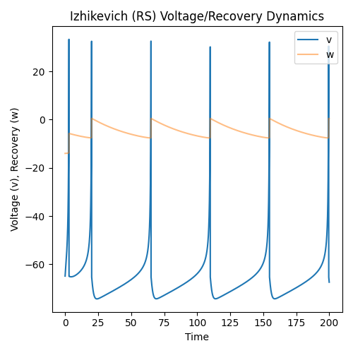
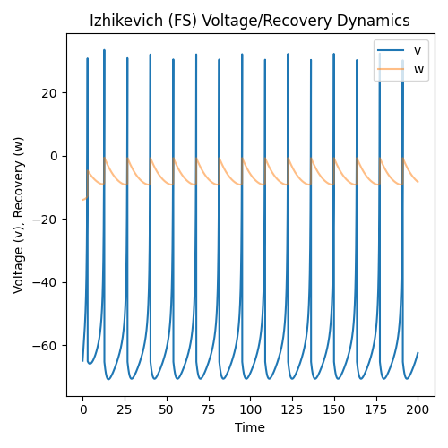
The plot above, which you can modify slightly yourself to include the neuronal type tag “RS” like we do, actually depicts the dynamics for a specific type of spiking neuron called the “regular spiking” (RS) neuron (also the default configuration for ngc-learn’s neuronal cell implementation), which is only one of several kinds of neurons you can emulate with Izhikevich’s dynamics implemented in ngc-learn. Try modifying the exposed Izhikevich cell hyper-parameters above and setting them to particular values (such as those noted in the component’s documentation) to recreate other possible neuron types. For example, to obtain a “fast spiking” (FS) neuronal cell, all you would need to do is modify the recovery variable’s time constant like so:
## FS cell configuration values
tau_w = 10. ## new recovery time constant
v_reset = -65. ## ngc-learn default
w_reset = 8.  ## ngc-learn default
coupling_factor = 0.2  ## ngc-learn default
to obtain a voltage/recovery dynamics plot like so (if you also modify the plot title of the plotting code accordingly):
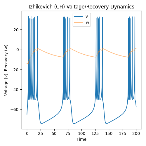
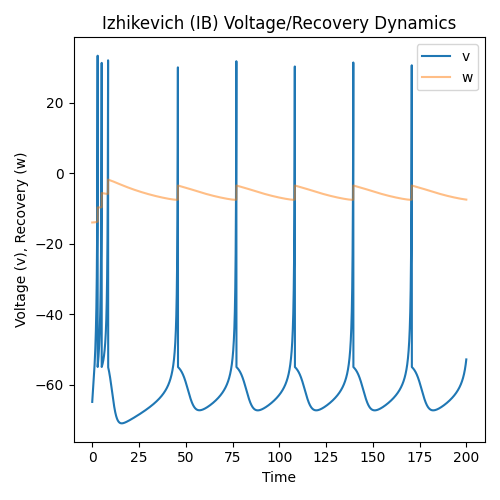
Three other well-known classes of neural behaviors are possible to easily simulate under the following hyper-parameter configurations (which produce the array of three plots similar to those shown near the bottom of this lesson), by simplifying modifying hyper-parameters according to the following:
Chattering (CH) neurons:
tau_w = 50.
v_reset = -50.
w_reset = 2.
coupling_factor=0.2
Intrinsically bursting (IB) neurons:
tau_w = 50.
v_reset = -55.
w_reset = 4.
coupling_factor=0.2
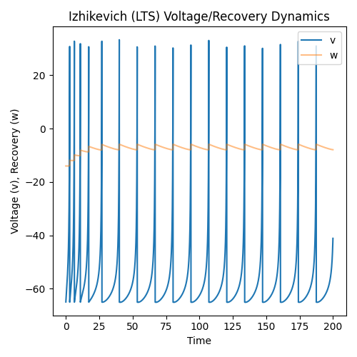
Low-threshold spiking (LTS) neurons:
tau_w = 50.
v_reset = -65.
w_reset = 2.
coupling_factor = 0.25
The above three hyper-parameter settings produce, from top-to-bottom, the plots shown below (from left-to-right):
|
|
|
References
[1] Izhikevich, Eugene M. “Simple model of spiking neurons.” IEEE Transactions on neural networks 14.6 (2003): 1569-1572.