Lecture 3A: The Rate Cell Model
Graded neurons are one of the main classes/collections of cell components in ngc-learn. These specifically offer cell models that operate under real-valued dynamics – in other words, they do not spike or use discrete pulse-like values in their operation. These are useful for building biophysical systems that evolve under continuous, time-varying dynamics, e.g., continuous-time recurrent neural networks, various kinds of predictive coding circuit models, as well as for continuous components in discrete systems, e.g. electrical current differential equations in spiking networks.
In this tutorial, we will study one of ngc-learn’s workhorse in-built graded cell components, the rate cell (RateCell).
Creating and Using a Rate Cell
Instantiating the Rate Cell
Let’s go ahead and set up the controller for this lesson’s simulation, where we will a dynamical system with only a single component, specifically the rate-cell (RateCell). Let’s start with the file’s header (or import statements):
from jax import numpy as jnp, random, jit

from ngclearn import Context, MethodProcess
## import model-specific elements
from ngclearn.components.neurons.graded.rateCell import RateCell
and move on to constructing the one component model:
## create seeding keys (JAX-style)
dkey = random.PRNGKey(1234)
dkey, *subkeys = random.split(dkey, 2)

dt = 1.  # ms # integration time constant
tau_m = 10.  # ms ## membrane time constant
act_fx = "unit_threshold"
gamma = 1.

with Context("Model") as model:  ## model/simulation definition
    ## instantiate components (like cells)
    cell = RateCell(
        "z0", n_units=1, tau_m=tau_m, act_fx=act_fx, prior=("gaussian", gamma), integration_type="euler",
        key=subkeys[0]
    )

    ## instantiate desired core commands that drive the simulation
    advance_process = (MethodProcess("advance")
                       >> cell.advance_state)
    reset_process = (MethodProcess("reset")
                     >> cell.reset)


## instantiate utility commands
def clamp(x):
    cell.j.set(x)
A notable argument to the rate-cell, beyond some of its differential equation constants (tau_m and gamma), is its activation function choice (default is the identity), which we have chosen to be a discrete pulse emitting function known as the unit_threshold (which outputs a value of one for any input that exceeds the threshold of one and zero for anything else).
Mathematically, under the hood, a rate-cell evolves according to the ordinary differential equation (ODE):
where \(\mathbf{x}\) is external input signal and \(\mathbf{x}_{td}\) (default value is zero) is an optional additional input pressure signal (td stands for “top-down”, its name motivated by predictive coding literature).
A good way to understand this equation is in the context of two examples:
in a biophysically more realistic spiking network, \(\mathbf{x}\) is the total electrical input into the cell from multiple injections produced by transmission across synapses (\(\mathbf{x}_{td} = 0\))) and the \(\text{prior}\) is set to
gaussian(\(\gamma = 1\)), yielding the equation \(\tau_m \frac{\partial \mathbf{z}}{\partial t} = -\mathbf{z} + \mathbf{x}\) for a simple model of synaptic conductance, andin a predictive coding circuit, \(\mathbf{x}\) is the sum of input projections (or messages) passed from a “lower” layer/group of neurons while \(\mathbf{x}_{td}\) is set to be the sum of (top-down) pressures produced by an “upper” layer/group such as the value of a pair of nearby error neurons multiplied by \(-1\).[1] In this example, \(0 \leq \gamma \leq 1\) and \(\text{prior}\) could be set to one of any kind of kurtotic distribution to induce a soft form of sparsity in the dynamics, e.g., such as “cauchy” for the Cauchy distribution.
Simulating a Rate Cell
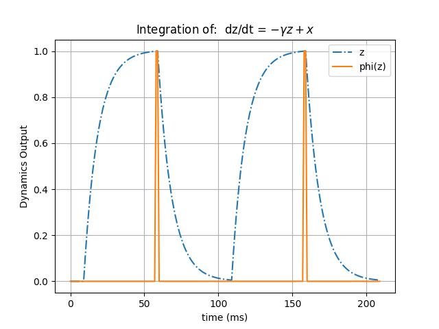
Given our single rate-cell dynamical system above, let us write some code to use our Rate node and visualize its dynamics by feeding into it a pulse current (a piecewise input function that is an alternating sequence of intervals of where nothing is input and others where a non-zero value is input) for a small period of time (dt * T = 1 * 210 ms). Specifically, we can plot the input current, the neuron’s linear rate activity z and its nonlinear activity phi(z) as follows:
# create a synthetic electrical pulse current
current = jnp.concatenate(
    (jnp.zeros((1,10)),
     jnp.ones((1,50)) * 1.006,
     jnp.zeros((1,50)),
     jnp.ones((1,50)) * 1.006,
     jnp.zeros((1,50))), axis=1
)

lin_out = []
nonlin_out = []
t_values = []

reset_process.run()
t = 0.
for ts in range(current.shape[1]):
   j_t = jnp.expand_dims(current[0,ts], axis=0) ## get data at time ts
   clamp(j_t)
   advance_process.run(t=ts*1., dt=dt)
   t_values.append(t)
   t += dt ## advance time forward by dt milliseconds

   ## naively extract simple statistics at time ts and print them to I/O
   linear_z = cell.z.get()
   nonlinear_z = cell.zF.get()
   lin_out.append(linear_z)
   nonlin_out.append(nonlinear_z)
   print("\r {}: s {} ; v {}".format(ts, linear_z, nonlinear_z), end="")
print()

import numpy as np
lin_out = np.squeeze(np.asarray(lin_out))
nonlin_out = np.squeeze(np.asarray(nonlin_out))
t_values = np.squeeze(np.asarray(t_values))

import matplotlib #.pyplot as plt
matplotlib.use('Agg')
import matplotlib.pyplot as plt
cmap = plt.cm.jet

fig, ax = plt.subplots()

zLin = ax.plot(t_values, lin_out, '-.', color='C0')
zNLin = ax.plot(t_values, nonlin_out, color='C1') #, alpha=.5)

ax.set(xlabel='time (ms)', ylabel='Dynamics Output',
       title='Integration of:  dz/dt = $-\gamma z + x$')
ax.legend([zLin[0],zNLin[0]],['z','phi(z)'])
ax.grid()
fig.savefig("rate_cell_integration.jpg")
which should yield a dynamics plot similar to the one below: