Lecture 3B: Error Cell Models

Error cells are a particularly useful component cell that offers a simple and fast way of computing mismatch signals, i.e., error values that compare a target value against a predicted value. In predictive coding literature, mismatch signals are often called “error neurons” and oftentimes are formulated as explicit cellular constructs that focus on computing the requisite difference values. In ngc-learn, error neuron component functionality has been in-built to readily allow construction of biophysical models that require mismatch signals, ranging from predictive coding circuitry to error-driven learning in spiking neural networks (see the ngc-museum for key examples of where error neurons come into play). In this lesson, we will briefly review one of the most commonly used ones – the Gaussian error cell.

Calculating Mismatch Values with the Gaussian Error Cell

The Gaussian error cell, much like most error neurons, is in fact a derived calculation when considering a cost function. Specifically, this error cell component inherits its name from the fact that it is producing output values akin to the first derivatives of a Gaussian log likelihood function. In neurobiological modeling, it is often useful to have the worked-out derivatives of the cost functions one might hypothesize that groups of neurons might be computing/optimizing, a setup that has yielded derivation of a wide plethora of learning rules in the biological credit assignment literature [1], most notably the prediction errors that drive the message passing scheme of mechanistic models of predictive coding [2].

In ngc-learn, error cell components are meant to produce not only the relevant partial derivative signals but also the local cost function value associated with them, since, again, error neurons are typically derived from some sort of objective. Furthermore, many of these kinds of neuronal cells can be treated as fast “fixed-point” computations, i.e., they do not have to adhere to dynamics dictated by ordinary differential equations[1], making them easy plug-in modules for the dynamical systems you might design.

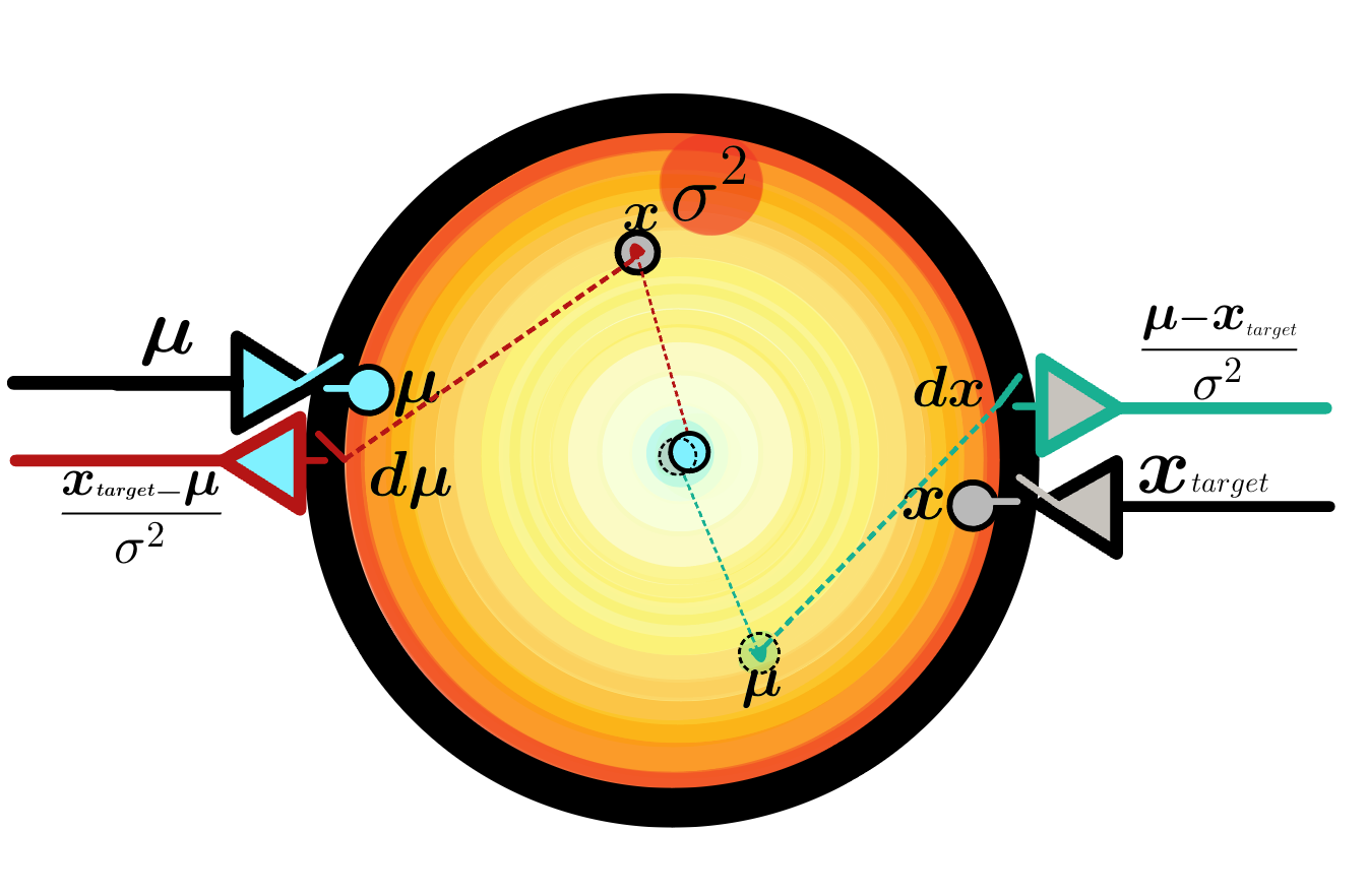
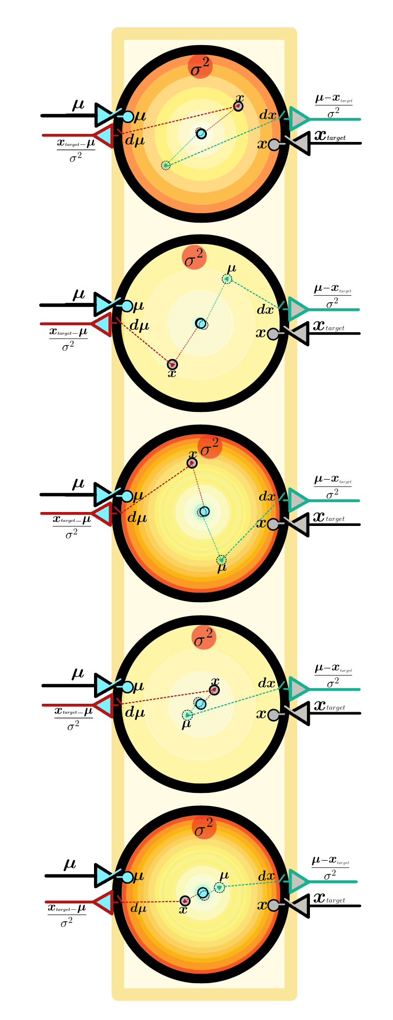
From a coding point-of-view, in-built error cell components can be imported and used in your models just like any other component; all that one needs to be aware of is the error cell compartment structure as these can produce different values that might be of interest depending on what the modeler wants to achieve. An in-built error cell component typically has at least five key components worth noting:

1. L – the local loss that this cell represents, essentially L = loss(target, mu);

2. mu – the prediction signal that this cell receives;

3. target – the target signal that this cell receives and compares to;

4. dmu – the partial derivative signal of L with respect to mu;

5. dtarget – the partial derivative signal of L with respect to target.

Let’s go ahead and import the GaussianErrorCell and see what it does, assuming we have a prediction vector guess produced from somewhere else (such as the output of another component or another model) and a target vector answer we wish that prediction could have been (which could also be the output of another component or another model). The code you would write amounts to the below:

from jax import numpy as jnp, jit

from ngclearn import Context, MethodProcess
## import model-specific mechanisms
from ngclearn.components.neurons.graded.gaussianErrorCell import GaussianErrorCell

dt = 1.  # ms # integration time constant
T = 5  ## number time steps to simulate

with Context("Model") as model:
    cell = GaussianErrorCell("z0", n_units=3)

    advance_process = (MethodProcess("advance_proc")
                       >> cell.advance_state)
    reset_process = (MethodProcess("reset_proc")
                     >> cell.reset)

## set up non-compiled utility commands
def clamp(x, y):
    ## error cells have two key input compartments; a "mu" and a "target"
    cell.mu.set(x)
    cell.target.set(y)
    

guess = jnp.asarray([[-1., 1., 1.]], jnp.float32)  ## the produced guess or prediction
answer = jnp.asarray([[1., -1., 1.]], jnp.float32)  ## what we wish the guess had been

reset_process.run() 
for ts in range(T):
    clamp(guess, answer)
    advance_process.run(t=ts * 1., dt=dt) 
    ## extract compartment values of interest
    dmu = cell.dmu.get()
    dtarget = cell.dtarget.get()
    loss = cell.L.get()
    ## print compartment values to I/O
    print("{} |  dmu: {}  dtarget: {}  loss: {} ".format(ts, dmu, dtarget, loss))

which should yield the following output:

0 |  dmu: [[ 2. -2.  0.]]  dtarget: [[-2.  2. -0.]]  loss: -4.0
1 |  dmu: [[ 2. -2.  0.]]  dtarget: [[-2.  2. -0.]]  loss: -4.0
2 |  dmu: [[ 2. -2.  0.]]  dtarget: [[-2.  2. -0.]]  loss: -4.0
3 |  dmu: [[ 2. -2.  0.]]  dtarget: [[-2.  2. -0.]]  loss: -4.0
4 |  dmu: [[ 2. -2.  0.]]  dtarget: [[-2.  2. -0.]]  loss: -4.0

where we see that the loss makes sense if we consider that the Gaussian log likelihood is being computed (under the assumption of a fixed scalar unit variance/standard deviation – which means we recover squared error; in other words, the cell effectively computes the loss: L = -(1/2) sum_j [(answer_j - guess-j)^2] = -0.5 * ((1 - -1)^2 + (-1 - 1)^2 + 0) = -4 where j indexes a particular dimension of the vector answer or guess). Note that since the prediction guess and target answer are fixed across time, running the Gaussian error for five steps of simulation time yield the same loss and partial derivatives. Finally, observe that dmu is the partial derivative of the cell’s local cost function with respect to the prediction/guess mu while dtarget is the partial derivative of the cell’s cost with respect to the target/answer target.

Other error cells, representing other types of distributions/loss functionals are possible with the error cell framework; all that a designer of a new custom component needs to mathematically consider is if they can provide the scalar loss signal that takes in prediction and target vectors as well as values for the partial derivatives with respect to the predictions and targets (note that these derivative signals, in principle, do not even have to be exact derivatives so long as they represent a means of traversing the flow of the cost function, finding local minima or maxima.)

References

[1] Ororbia, Alexander G. “Brain-inspired machine intelligence: A survey of neurobiologically-plausible credit assignment.” arXiv preprint arXiv:2312.09257 (2023).
[2] Rao, Rajesh PN, and Dana H. Ballard. “Predictive coding in the visual cortex: a functional interpretation of some extra-classical receptive-field effects.” Nature neuroscience 2.1 (1999).
[3] Bogacz, Rafal. “A tutorial on the free-energy framework for modelling perception and learning.” Journal of mathematical psychology 76 (2017).

---

[1]

Note that, technically, error neurons do not have to be formulated as immediate fixed-point computations and can be framed in terms of differential equations as any other neuron component. See [3] for details on error neuron dynamics in this case.