Lecture 4A: Dynamic Synapses and Conductance
In this lesson, we will study dynamic synapses, or synaptic cable components in ngc-learn that evolve on fast time-scales in response to their pre-synaptic inputs. These types of chemical synapse components are useful for modeling time-varying conductance which ultimately drives electrical current input into neuronal units (such as spiking cells). Here, we will learn how to build three important types of dynamic synapses in ngc-learn – the exponential, the alpha, and the double-exponential synapse – and visualize the time-course of their resulting conductances. In addition, we will then construct and study a small neuronal circuit involving a leaky integrator that is driven by exponential synapses relaying pulses from an excitatory and an inhibitory population of Poisson input encoding cells.
Synaptic Conductance Modeling
Synapse models are typically used to model the post-synaptic response produced by action potentials (or pulses) at a pre-synaptic terminal. Assuming an electrical response (as opposed to a chemical one, e.g., an influx of calcium), such models seek to emulate the time-course of what is known as post-synaptic receptor conductance. Note that these dynamic synapse models will end being a bit more sophisticated than the strength value matrices we might initially employ (as in synapse components such as the DenseSynapse).
Building a dynamic synapse can be done by importing the exponential synapse,
the double-exponential synapse, or the alpha synapse from ngc-learn’s in-built components and setting them up within a model context for easy analysis. Go ahead and create a Python script named probe_dynamic_synapses.py to place
the code you will write within.
For the first part of this lesson, we will import all three dynamic synapse models and compare their behavior.
This can be done as follows (using the meta-parameters we provide in the code block below to ensure reasonable dynamics):
from jax import numpy as jnp, random, jit
from ngclearn import Context, MethodProcess
from ngclearn.components import ExponentialSynapse, AlphaSynapse, DoubleExpSynapse
from ngclearn.utils.distribution_generator import DistributionGenerator


dkey = random.PRNGKey(1234) ## creating seeding keys for synapses
dkey, *subkeys = random.split(dkey, 6)
dt = 0.1 # ms ## integration time constant
T = 8. # ms ## total duration time

## ---- build a dual-synapse system ----
with Context("dual_syn_system") as ctx:
    Wexp = ExponentialSynapse( ## exponential dynamic synapse
        name="Wexp", shape=(1, 1), tau_decay=3., g_syn_bar=1., syn_rest=0., resist_scale=1.,
        weight_init=DistributionGenerator.constant(value=1.), key=subkeys[0]
    )
    Walpha = AlphaSynapse( ## alpha dynamic synapse
        name="Walpha", shape=(1, 1), tau_decay=1., g_syn_bar=1., syn_rest=0., resist_scale=1.,
        weight_init=DistributionGenerator.constant(value=1.), key=subkeys[0]
    )
    Wexp2 = DoubleExpSynapse(
        name="Wexp2", shape=(1, 1), tau_rise=1., tau_decay=3., g_syn_bar=1., syn_rest=0., resist_scale=1.,
        weight_init=DistributionGenerator.constant(value=1.), key=subkeys[0]
    )

    ## set up basic simulation process calls
    advance_process = (MethodProcess("advance_proc")
                       >> Wexp.advance_state
                       >> Walpha.advance_state
                       >> Wexp2.advance_state)

    reset_process = (MethodProcess("reset_proc")
                     >> Wexp.reset
                     >> Walpha.reset
                     >> Wexp2.reset)
where we notice in the above we have instantiated three different kinds of chemical synapse components that we will run side-by-side in order to extract their produced conductance values in response to the exact same input stream. For both the exponential and the alpha synapse, there are at least three important hyper-parameters to configure:
tau_decay(\(\tau_{\text{decay}}\)): the synaptic conductance decay time constant (for the double-exponential synapse, we also havetau_rise);g_syn_bar(\(\bar{g}_{\text{syn}}\)): the maximal conductance value produced by each pulse transmitted across this synapse; and,syn_rest(\(E_{rest}\)): the (post-synaptic) reversal potential for this synapse – note that this value determines the direction of current flow through the synapse, yielding a synapse with an excitatory nature for non-negative values ofsyn_restor a synapse with an inhibitory nature for negative values ofsyn_rest.
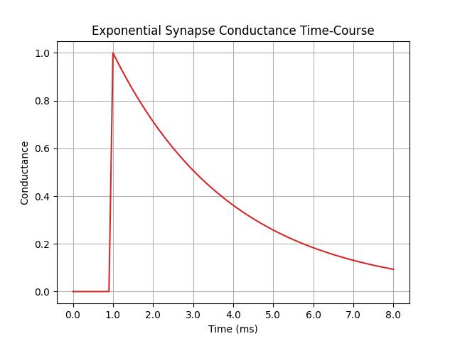
The flow of electrical current from a pre-synaptic neuron to a post-synaptic one is often modeled under the assumption that pre-synaptic pulses result in impermanent (transient; lasting for a short period of time) changes in the conductance of a post-synaptic neuron. As a result, the resulting conductance dynamics \(g_{\text{syn}}(t)\) – or the effect (conductance changes in the post-synaptic membrane) of a transmitter binding to and opening post-synaptic receptors – of each of the synapses that you have built above can be simulated in ngc-learn according to one or more ordinary differential equations (ODEs), which themselves iteratively model different waveform equations of the time-course of synaptic conductance. For the exponential synapse, the dynamics adhere to the following ODE:
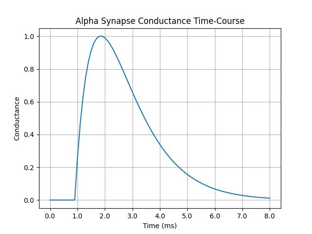
where the conductance (for a post-synaptic unit) output of this synapse is driven by a sum over all of its incoming pre-synaptic spikes; this ODE means that pre-synaptic spikes are filtered via an exponential kernel (i.e., a low-pass filter). On the other hand, for the alpha synapse, the dynamics adhere to the following coupled set of ODEs:
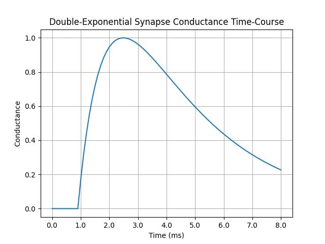
where \(h_{\text{syn}}(t)\) is an intermediate variable that operates in service of driving the conductance variable \(g_{\text{syn}}(t)\) itself. The double-exponential (or difference of exponentials) synapse model looks similar to the alpha synapse except that the rise and fall/decay of its conductance dynamics are set separately using two different time constants, i.e., \(\tau_{\text{rise}}\) and \(\tau_{\text{decay}}\), as follows:
Finally, we seek model the electrical current that results from some amount of neurotransmitter in previous time steps. Thus, for both any of these three synapses, the changes in conductance are finally converted (via Ohm’s law) to electrical current to produce the final derived variable \(j_{\text{syn}}(t)\):
where \(E_{\text{rev}}\) is the post-synaptic reverse potential of the ion channels that mediate the synaptic current; this is typically set to \(E_{\text{rev}} = 0\) (millivolts; mV)for the case of excitatory changes and \(E_{\text{rev}} = -75\) (mV) for the case of inhibitory changes. \(v(t)\) is the voltage/membrane potential of the post-synaptic the synaptic cable wires to, meaning that the conductance models above are voltage-dependent (in ngc-learn, if you want voltage-independent conductance, then set syn_rest = None).
Examining the Conductances of Dynamic Synapses
We can track and visualize the conductance outputs of our different dynamic synapses by running a stream of controlled pre-synaptic pulses. Specifically, we will observe the output behavior of each in response to a sparse stream, eight milliseconds in length, where only a single spike is emitted at one millisecond. To create the simulation of a single input pulse stream, you can write the following code:
time_span = []
g = []
ga = []
gexp2 = []
reset_process.run()
Tsteps = int(T/dt) + 1
for t in range(Tsteps):
    s_t = jnp.zeros((1, 1))
    if t * dt == 1.: ## pulse at 1 ms
        s_t = jnp.ones((1, 1))
    Wexp.inputs.set(s_t)
    Walpha.inputs.set(s_t)
    Wexp.v.set(Wexp.v.get() * 0)
    Wexp2.inputs.set(s_t)
    Walpha.v.set(Walpha.v.get() * 0)
    Wexp2.v.set(Wexp2.v.get() * 0)
    advance_process.run(t=t * dt, dt=dt)

    print(f"\r g = {Wexp.g_syn.get()}  ga = {Walpha.g_syn.get()}  gexp2 = {Wexp2.g_syn.get()}", end="")
    g.append(Wexp.g_syn.get())
    ga.append(Walpha.g_syn.get())
    gexp2.append(Wexp2.g_syn.get())
    time_span.append(t) #* dt)
print()
g = jnp.squeeze(jnp.concatenate(g, axis=1))
g = g/jnp.amax(g)
ga = jnp.squeeze(jnp.concatenate(ga, axis=1))
ga = ga/jnp.amax(ga)
gexp2 = jnp.squeeze(jnp.concatenate(gexp2, axis=1))
gexp2 = gexp2/jnp.amax(gexp2)
Note that we further normalize the conductance trajectories of all synapses to lie within the range of \([0, 1]\), primarily for visualization purposes. Finally, to visualize the conductance time-course of the synapses, you can write the following:
import matplotlib #.pyplot as plt
matplotlib.use('Agg')
import matplotlib.pyplot as plt
cmap = plt.cm.jet

time_ticks = []
time_labs = []
for t in range(Tsteps):
    if t % 10 == 0:
        time_ticks.append(t)
        time_labs.append(f"{t * dt:.1f}")

## ---- plot the exponential synapse conductance time-course ----
fig, ax = plt.subplots()

gvals = ax.plot(time_span, g, '-', color='tab:red')
#plt.xticks(time_span, time_labs)
ax.set_xticks(time_ticks, time_labs)
ax.set(xlabel='Time (ms)', ylabel='Conductance',
      title='Exponential Synapse Conductance Time-Course')
ax.grid(which="major")
fig.savefig("exp_syn.jpg")
plt.close()

## ---- plot the alpha synapse conductance time-course ----
fig, ax = plt.subplots()

gvals = ax.plot(time_span, ga, '-', color='tab:blue')
#plt.xticks(time_span, time_labs)
ax.set_xticks(time_ticks, time_labs)
ax.set(xlabel='Time (ms)', ylabel='Conductance',
      title='Alpha Synapse Conductance Time-Course')
ax.grid(which="major")
fig.savefig("alpha_syn.jpg")
plt.close()

## ---- plot the double-exponential synapse conductance time-course ----
fig, ax = plt.subplots()

gvals = ax.plot(time_span, gexp2, '-', color='tab:blue')
#plt.xticks(time_span, time_labs)
ax.set_xticks(time_ticks, time_labs)
#plt.vlines(x=[0, 10, 20, 30, 40, 50, 60, 70, 80], ymin=-0.2, ymax=1.2, colors='gray', linestyles='dashed') #, label='Vertical Lines')
ax.set(xlabel='Time (ms)', ylabel='Conductance',
      title='Double-Exponential Synapse Conductance Time-Course')
ax.grid(which="major")
fig.savefig("exp2_syn.jpg")
plt.close()
which should produce and save three plots to disk. You can then compare and contrast the plots of the exponential, alpha synapse, and double-exponential conductance trajectories:
|
|
|
Note that the alpha synapse (right figure) would produce a more realistic fit to recorded synaptic currents (as it attempts to model the rise and fall of current in a less simplified manner) at the cost of extra compute, given it uses two ODEs to emulate conductance, as opposed to the faster yet less-biophysically-realistic exponential synapse (left figure).
Excitatory-Inhibitory Driven Dynamics
For this next part of the lesson, create a new Python script named sim_ei_dynamics.py for the next portions of code
you will write.
Let’s next examine a more interesting use-case of the above dynamic synapses – modeling excitatory (E) and inhibitory (I)
pressures produced by different groups of pre-synaptic spike trains. This allows us to examine a very common
and often-used conductance model that is paired with spiking cells such as the leaky integrate-and-fire (LIF). Specifically,
we seek to simulate the following post-synaptic conductance dynamics for a single LIF unit:
where \(g_{L}\) is the leak conductance value for the post-synaptic LIF, \(g_{E}(t)\) is the post-synaptic conductance produced by excitatory pre-synaptic spike trains (with excitatory synaptic reverse potential \(E_{E}\)), and \(g_{I}(t)\) is the post-synaptic conductance produced by inhibitory pre-synaptic spike trains (with inhibitory synaptic reverse potential \(E_{I}\)). Note that the first term of the above ODE is the normal leak portion of the LIF’s standard dynamics (scaled by conductance factor \(g_{L}\)) and the last two terms of the above ODE can be modeled each separately with a dynamic synapse. To differentiate between excitatory and inhibitory conductance changes, we will just configure a different reverse potential for each to induce either excitatory (i.e., \(E_{\text{syn}} = E_{E} = 0\) mV) or inhibitory (i.e., \(E_{\text{syn}} = E_{I} = -80\) mV) pressure/drive.
We will specifically model the excitatory and inhibitory conductance changes using exponential synapses and the input spike trains for each with Poisson encoding cells; in other words, two different groups of Poisson cells will be wired to a single LIF cell via exponential dynamic synapses. The code for doing this is as follows:
from jax import numpy as jnp, random, jit
from ngclearn import Context, MethodProcess
from ngclearn.operations import Summation
from ngclearn.components import ExponentialSynapse, PoissonCell, LIFCell
from ngclearn.utils.distribution_generator import DistributionGenerator

## create seeding keys
dkey = random.PRNGKey(1234)
dkey, *subkeys = random.split(dkey, 6)

## simulation properties
dt = 0.1 # ms
T = 1000. # ms ## total duration time

## post-syn LIF cell properties
tau_m = 10.
g_L = 10.
v_rest = -75.
v_thr = -55.

## excitatory group properties
exc_freq = 10. # Hz
n_exc = 80
g_e_bar = 2.4
tau_syn_exc = 2.
E_rest_exc = 0.

## inhibitory group properties
inh_freq = 10. # Hz
n_inh = 20
g_i_bar = 2.4
tau_syn_inh = 5.
E_rest_inh = -80.

Tsteps = int(T/dt)

## ---- build a simple E-I spiking circuit ----
with Context("ei_snn") as ctx:
    pre_exc = PoissonCell("pre_exc", n_units=n_exc, target_freq=exc_freq, key=subkeys[0]) ## pre-syn excitatory group
    pre_inh = PoissonCell("pre_inh", n_units=n_inh, target_freq=inh_freq, key=subkeys[1]) ## pre-syn inhibitory group
    Wexc = ExponentialSynapse( ## dynamic synapse between excitatory group and LIF
        name="Wexc", shape=(n_exc,1), tau_decay=tau_syn_exc, g_syn_bar=g_e_bar, syn_rest=E_rest_exc, resist_scale=1./g_L,
        weight_init=DistributionGenerator.constant(value=1.), key=subkeys[2]
    )
    Winh = ExponentialSynapse( ## dynamic synapse between inhibitory group and LIF
        name="Winh", shape=(n_inh, 1), tau_decay=tau_syn_inh, g_syn_bar=g_i_bar, syn_rest=E_rest_inh, resist_scale=1./g_L,
        weight_init=DistributionGenerator.constant(value=1.), key=subkeys[2]
    )
    post_exc = LIFCell( ## post-syn LIF cell
        "post_exc", n_units=1, tau_m=tau_m, resist_m=1., thr=v_thr, v_rest=v_rest, conduct_leak=1., v_reset=-75.,
        tau_theta=0., theta_plus=0., refract_time=2., key=subkeys[3]
    )

    pre_exc.outputs >> Wexc.inputs
    pre_inh.outputs >> Winh.inputs
    post_exc.v >> Wexc.v ## couple voltage to exc synapse
    post_exc.v >> Winh.v ## couple voltage to inh synapse
    Summation(Wexc.i_syn, Winh.i_syn) >> post_exc.j ## sum together excitatory & inhibitory pressures

    advance_process = (MethodProcess("advance_proc")
                       >> pre_exc.advance_state
                       >> pre_inh.advance_state
                       >> Wexc.advance_state
                       >> Winh.advance_state
                       >> post_exc.advance_state)

    reset_process = (MethodProcess("reset_proc")
                     >> pre_exc.reset
                     >> pre_inh.reset
                     >> Wexc.reset
                     >> Winh.reset
                     >> post_exc.reset)
Examining the Simple Spiking Circuit’s Behavior
To run the above spiking circuit, we then write the next block of code (making sure to track/store the resulting membrane potential and pulse values emitted by the post-synaptic LIF):
volts = []
time_span = []
spikes = []

reset_process.run()
pre_exc.inputs.set(jnp.ones((1, n_exc)))
pre_inh.inputs.set(jnp.ones((1, n_inh)))
post_exc.v.set(post_exc.v.get() * 0 - 65.) ## initial condition for LIF is -65 mV
volts.append(post_exc.v.get())
time_span.append(0.)
Tsteps = int(T/dt) + 1
for t in range(1, Tsteps):
    advance_process.run(t=t * dt, dt=dt)
    print(f"\r v {post_exc.v.get()}", end="")
    volts.append(post_exc.v.get())
    spikes.append(post_exc.s.get())
    time_span.append(t) #* dt)
print()
volts = jnp.squeeze(jnp.concatenate(volts, axis=1))
spikes = jnp.squeeze(jnp.concatenate(spikes, axis=1))
from which we may then write the following plotting code to visualize the post-synaptic LIF unit’s membrane potential time-course along with any spikes it might have produced in response to the pre-synaptic spike trains:
import matplotlib
matplotlib.use('Agg')
import matplotlib.pyplot as plt
cmap = plt.cm.jet

time_ticks = []
time_labs = []
time_ticks.append(0)
time_labs.append(f"{0.}")
tdiv = 1000
for t in range(Tsteps):
    if t % tdiv == 0:
        time_ticks.append(t)
        time_labs.append(f"{t * dt:.0f}")

fig, ax = plt.subplots()

volt_vals = ax.plot(time_span, volts, '-.', color='tab:red')
stat = jnp.where(spikes > 0.)
indx = (stat[0] * 1. - 1.).tolist()
v_thr_below = -0.75
v_thr_above = 2.
spk = ax.vlines(x=indx, ymin=v_thr-v_thr_below, ymax=v_thr+v_thr_above, colors='black', ls='-', lw=2)
_v_thr = v_thr
ax.hlines(y=_v_thr, xmin=0., xmax=time_span[-1], colors='blue', ls='-.', lw=2)

ax.set(xlabel='Time (ms)', ylabel='Voltage',
      title='Exponential Synapse LIF')
ax.grid()
fig.savefig("ei_circuit_dynamics.jpg")
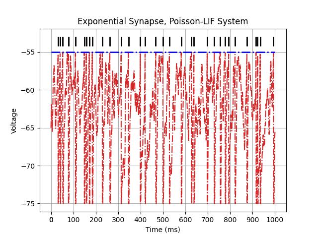
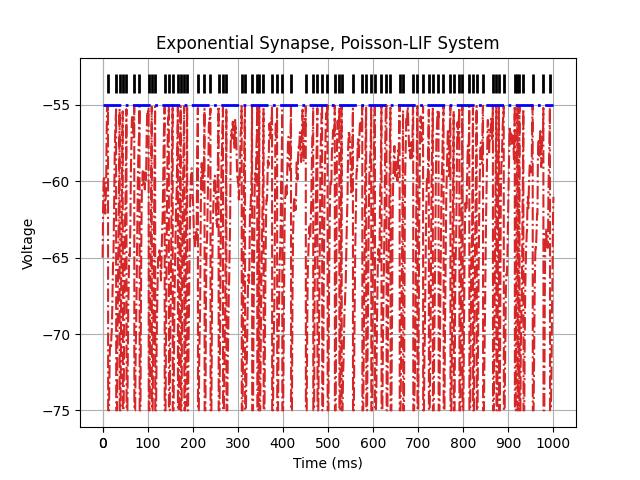
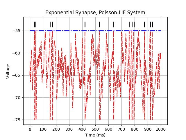
which should produce a figure depicting dynamics similar to the one below. Black tick marks indicate post-synaptic pulses whereas the horizontal dashed blue shows the LIF unit’s voltage threshold.
|
Notice that the above shows the behavior of the post-synaptic LIF in response to the integration of pulses coming from two Poisson spike trains both at rates of \(10\) Hz (since both exc_freq and inh_freq have been set to ten). Messing with the frequencies of the excitatory and inhibitory pulse trains can lead to sparser or denser post-synaptic spike outputs. For instance, if we increase the frequency of the excitatory train to \(15\) Hz (keeping the inhibitory one at \(10\) Hz), we get a denser post-synaptic output pulse pattern as in the left figure below. In contrast, if we instead increase the inhibitory frequency to \(30\) Hz (keeping the excitatory at \(10\) Hz), we obtain a sparser post-synaptic output pulse train as in the right figure below.
|
|
References
[1] Sterratt, David, et al. Principles of computational modelling in neuroscience. Cambridge university
press, 2023.
[2] Roth, Arnd, and Mark CW van Rossum. “Modeling synapses.” Computational modeling methods for neuroscientists 6.139 (2009): 700.